10 Truncation Error Analysis
Truncation error analysis provides a widely applicable framework for analyzing the accuracy of finite difference schemes. This type of analysis can also be used for finite element and finite volume methods if the discrete equations are written in finite difference form. The result of the analysis is an asymptotic estimate of the error in the scheme on the form \(Ch^r\), where \(h\) is a discretization parameter (\(\Delta t\), \(\Delta x\), etc.), \(r\) is a number, known as the convergence rate, and \(C\) is a constant, typically dependent on the derivatives of the exact solution.
Knowing \(r\) gives understanding of the accuracy of the scheme. But maybe even more important, a powerful verification method for computer codes is to check that the empirically observed convergence rates in experiments coincide with the theoretical value of \(r\) found from truncation error analysis.
The analysis can be carried out by hand, by symbolic software, and also numerically. All three methods will be illustrated. From examining the symbolic expressions of the truncation error we can add correction terms to the differential equations in order to increase the numerical accuracy.
In general, the term truncation error refers to the discrepancy that arises from performing a finite number of steps to approximate a process with infinitely many steps. The term is used in a number of contexts, including truncation of infinite series, finite precision arithmetic, finite differences, and differential equations. We shall be concerned with computing truncation errors arising in finite difference formulas and in finite difference discretizations of differential equations.
10.1 Abstract problem setting
Consider an abstract differential equation \[ \mathcal{L}(u)=0, \] where \(\mathcal{L}(u)\) is some formula involving the unknown \(u\) and its derivatives. One example is \(\mathcal{L}(u)=u'(t)+a(t)u(t)-b(t)\), where \(a\) and \(b\) are constants or functions of time. We can discretize the differential equation and obtain a corresponding discrete model, here written as \[ \mathcal{L}_{\Delta}(u) =0\tp \] The solution \(u\) of this equation is the numerical solution. To distinguish the numerical solution from the exact solution of the differential equation problem, we denote the latter by \(u_{\text{e}}\) and write the differential equation and its discrete counterpart as
\[\begin{align*} \mathcal{L}(u_{\text{e}})&=0,\\ \mathcal{L}_\Delta (u)&=0\tp \end{align*}\] Initial and/or boundary conditions can usually be left out of the truncation error analysis and are omitted in the following.
The numerical solution \(u\) is, in a finite difference method, computed at a collection of mesh points. The discrete equations represented by the abstract equation \(\mathcal{L}_\Delta (u)=0\) are usually algebraic equations involving \(u\) at some neighboring mesh points.
10.2 Error measures
A key issue is how accurate the numerical solution is. The ultimate way of addressing this issue would be to compute the error \(u_{\text{e}} - u\) at the mesh points. This is usually extremely demanding. In very simplified problem settings we may, however, manage to derive formulas for the numerical solution \(u\), and therefore closed form expressions for the error \(u_{\text{e}} - u\). Such special cases can provide considerable insight regarding accuracy and stability, but the results are established for special problems.
The error \(u_{\text{e}} -u\) can be computed empirically in special cases where we know \(u_{\text{e}}\). Such cases can be constructed by the method of manufactured solutions, where we choose some exact solution \(u_{\text{e}} = v\) and fit a source term \(f\) in the governing differential equation \(\mathcal{L}(u_{\text{e}})=f\) such that \(u_{\text{e}}=v\) is a solution (i.e., \(f=\mathcal{L}(v)\)). Assuming an error model of the form \(Ch^r\), where \(h\) is the discretization parameter, such as \(\Delta t\) or \(\Delta x\), one can estimate the convergence rate \(r\). This is a widely applicable procedure, but the validity of the results is, strictly speaking, tied to the chosen test problems.
Another error measure arises by asking to what extent the exact solution \(u_{\text{e}}\) fits the discrete equations. Clearly, \(u_{\text{e}}\) is in general not a solution of \(\mathcal{L}_\Delta(u)=0\), but we can define the residual \[ R = \mathcal{L}_\Delta(u_{\text{e}}), \] and investigate how close \(R\) is to zero. A small \(R\) means intuitively that the discrete equations are close to the differential equation, and then we are tempted to think that \(u^n\) must also be close to \(u_{\text{e}}(t_n)\).
The residual \(R\) is known as the truncation error of the finite difference scheme \(\mathcal{L}_\Delta(u)=0\). It appears that the truncation error is relatively straightforward to compute by hand or symbolic software without specializing the differential equation and the discrete model to a special case. The resulting \(R\) is found as a power series in the discretization parameters. The leading-order terms in the series provide an asymptotic measure of the accuracy of the numerical solution method (as the discretization parameters tend to zero). An advantage of truncation error analysis, compared to empirical estimation of convergence rates, or detailed analysis of a special problem with a mathematical expression for the numerical solution, is that the truncation error analysis reveals the accuracy of the various building blocks in the numerical method and how each building block impacts the overall accuracy. The analysis can therefore be used to detect building blocks with lower accuracy than the others.
Knowing the truncation error or other error measures is important for verification of programs by empirically establishing convergence rates. The forthcoming text will provide many examples on how to compute truncation errors for finite difference discretizations of ODEs and PDEs.
10.3 Truncation errors in finite difference formulas
The accuracy of a finite difference formula is a fundamental issue when discretizing differential equations. We shall first go through a particular example in detail and thereafter list the truncation error in the most common finite difference approximation formulas.
10.4 Example: The backward difference for \(u'(t)\)
Consider a backward finite difference approximation of the first-order derivative \(u'\): \[ \lbrack D_t^- u\rbrack^n = \frac{u^{n} - u^{n-1}}{\Delta t} \approx u'(t_n) \tp \tag{10.1}\] Here, \(u^n\) means the value of some function \(u(t)\) at a point \(t_n\), and \([D_t^-u]^n\) is the discrete derivative of \(u(t)\) at \(t=t_n\). The discrete derivative computed by a finite difference is, in general, not exactly equal to the derivative \(u'(t_n)\). The error in the approximation is \[ R^n = [D^-_tu]^n - u'(t_n)\tp \tag{10.2}\]
The common way of calculating \(R^n\) is to
- expand \(u(t)\) in a Taylor series around the point where the derivative is evaluated, here \(t_n\),
- insert this Taylor series in (10.2), and
- collect terms that cancel and simplify the expression.
The result is an expression for \(R^n\) in terms of a power series in \(\Delta t\). The error \(R^n\) is commonly referred to as the truncation error of the finite difference formula.
The Taylor series formula often found in calculus books takes the form \[ f(x+h) = \sum_{i=0}^\infty \frac{1}{i!}\frac{d^if}{dx^i}(x)h^i\tp \] In our application, we expand the Taylor series around the point where the finite difference formula approximates the derivative. The Taylor series of \(u^n\) at \(t_n\) is simply \(u(t_n)\), while the Taylor series of \(u^{n-1}\) at \(t_n\) must employ the general formula, \[\begin{align*} u(t_{n-1}) = u(t-\Delta t) &= \sum_{i=0}^\infty \frac{1}{i!}\frac{d^iu}{dt^i}(t_n)(-\Delta t)^i\\ & = u(t_n) - u'(t_n)\Delta t + {\half}u''(t_n)\Delta t^2 + \Oof{\Delta t^3}, \end{align*}\] where \(\Oof{\Delta t^3}\) means a power-series in \(\Delta t\) where the lowest power is \(\Delta t^3\). We assume that \(\Delta t\) is small such that \(\Delta t^p \gg \Delta t^q\) if \(p\) is smaller than \(q\). The details of higher-order terms in \(\Delta t\) are therefore not of much interest. Inserting the Taylor series above in the right-hand side of (10.2) gives rise to some algebra:
\[\begin{align*} [D_t^-u]^n - u'(t_n) &= \frac{u(t_n) - u(t_{n-1})}{\Delta t} - u'(t_n)\\ &= \frac{u(t_n) - (u(t_n) - u'(t_n)\Delta t + {\half}u''(t_n)\Delta t^2 + \Oof{\Delta t^3} )}{\Delta t} - u'(t_n)\\ &= -{\half}u''(t_n)\Delta t + \Oof{\Delta t^2} ), \end{align*}\] which is, according to (10.2), the truncation error: \[ R^n = - {\half}u''(t_n)\Delta t + \Oof{\Delta t^2} ) \tp \] The dominating term for small \(\Delta t\) is \(-{\half}u''(t_n)\Delta t\), which is proportional to \(\Delta t\), and we say that the truncation error is of first order in \(\Delta t\).
10.5 Example: The forward difference for \(u'(t)\)
We can analyze the approximation error in the forward difference \[ u'(t_n) \approx [D_t^+ u]^n = \frac{u^{n+1}-u^n}{\Delta t}, \] by writing \[ R^n = [D_t^+ u]^n - u'(t_n), \] and expanding \(u^{n+1}\) in a Taylor series around \(t_n\), \[ u(t_{n+1}) = u(t_n) + u'(t_n)\Delta t + {\half}u''(t_n)\Delta t^2 + \Oof{\Delta t^3} \tp \] The result becomes \[ R = {\half}u''(t_n)\Delta t + \Oof{\Delta t^2}, \] showing that also the forward difference is of first order.
10.6 Example: The central difference for \(u'(t)\)
For the central difference approximation, \[ u'(t_n)\approx [ D_tu]^n, \quad [D_tu]^n = \frac{u^{n+\half} - u^{n-\half}}{\Delta t}, \] we write \[ R^n = [ D_tu]^n - u'(t_n), \] and expand \(u(t_{n+\half})\) and \(u(t_{n-\half}\) in Taylor series around the point \(t_n\) where the derivative is evaluated. We have \[\begin{align*} u(t_{n+\half}) = &u(t_n) + u'(t_n)\half\Delta t + {\half}u''(t_n)(\half\Delta t)^2 + \\ & \frac{1}{6}u'''(t_n) (\half\Delta t)^3 + \frac{1}{24}u''''(t_n) (\half\Delta t)^4 + \\ & \frac{1}{120}u''''(t_n) (\half\Delta t)^5 + \Oof{\Delta t^6},\\ u(t_{n-\half}) = &u(t_n) - u'(t_n)\half\Delta t + {\half}u''(t_n)(\half\Delta t)^2 - \\ & \frac{1}{6}u'''(t_n) (\half\Delta t)^3 + \frac{1}{24}u''''(t_n) (\half\Delta t)^4 - \\ & \frac{1}{120}u'''''(t_n) (\half\Delta t)^5 + \Oof{\Delta t^6} \end{align*}\] Now, \[ u(t_{n+\half}) - u(t_{n-\half}) = u'(t_n)\Delta t + \frac{1}{24}u'''(t_n) \Delta t^3 + \frac{1}{960}u'''''(t_n) \Delta t^5 + \Oof{\Delta t^7} \tp \] By collecting terms in \([D_t u]^n - u'(t_n)\) we find the truncation error to be \[ R^n = \frac{1}{24}u'''(t_n)\Delta t^2 + \Oof{\Delta t^4}, \] with only even powers of \(\Delta t\). Since \(R\sim \Delta t^2\) we say the centered difference is of second order in \(\Delta t\).
10.7 Overview of leading-order error terms in finite difference formulas
Here we list the leading-order terms of the truncation errors associated with several common finite difference formulas for the first and second derivatives.
\[ \begin{split} \lbrack D_tu \rbrack^n &= \frac{u^{n+\half} - u^{n-\half}}{\Delta t} = u'(t_n) + R^n,\\ R^n &= \frac{1}{24}u'''(t_n)\Delta t^2 + \Oof{\Delta t^4} \end{split} \tag{10.3}\] \[ \begin{split} \lbrack D_{2t}u \rbrack^n &= \frac{u^{n+1} - u^{n-1}}{2\Delta t} = u'(t_n) + R^n,\\ R^n &= \frac{1}{6}u'''(t_n)\Delta t^2 + \Oof{\Delta t^4} \end{split} \tag{10.4}\] \[ \begin{split} \lbrack D_t^-u \rbrack^n &= \frac{u^{n} - u^{n-1}}{\Delta t} = u'(t_n) + R^n,\\ R^n &= -{\half}u''(t_n)\Delta t + \Oof{\Delta t^2} \end{split} \tag{10.5}\] \[ \begin{split} \lbrack D_t^+u \rbrack^n &= \frac{u^{n+1} - u^{n}}{\Delta t} = u'(t_n) + R^n,\\ R^n &= {\half}u''(t_n)\Delta t + \Oof{\Delta t^2} \end{split} \tag{10.6}\] \[ \begin{split} [\bar D_tu]^{n+\theta} &= \frac{u^{n+1} - u^{n}}{\Delta t} = u'(t_{n+\theta}) + R^{n+\theta},\\ R^{n+\theta} &= \half(1-2\theta)u''(t_{n+\theta})\Delta t - \frac{1}{6}((1 - \theta)^3 - \theta^3)u'''(t_{n+\theta})\Delta t^2 + \Oof{\Delta t^3} \end{split} \tag{10.7}\] \[ \begin{split} \lbrack D_t^{2-}u \rbrack^n &= \frac{3u^{n} - 4u^{n-1} + u^{n-2}}{2\Delta t} = u'(t_n) + R^n,\\ R^n &= -\frac{1}{3}u'''(t_n)\Delta t^2 + \Oof{\Delta t^3} \end{split} \tag{10.8}\] \[ \begin{split} \lbrack D_tD_t u \rbrack^n &= \frac{u^{n+1} - 2u^{n} + u^{n-1}}{\Delta t^2} = u''(t_n) + R^n,\\ R^n &= \frac{1}{12}u''''(t_n)\Delta t^2 + \Oof{\Delta t^4} \end{split} \tag{10.9}\]
It will also be convenient to have the truncation errors for various means or averages. The weighted arithmetic mean leads to
\[ \begin{split} [\overline{u}^{t,\theta}]^{n+\theta} & = \theta u^{n+1} + (1-\theta)u^n = u(t_{n+\theta}) + R^{n+\theta}, \\ R^{n+\theta} &= {\half}u''(t_{n+\theta})\Delta t^2\theta (1-\theta) + \Oof{\Delta t^3}\tp \end{split} \tag{10.10}\] The standard arithmetic mean follows from this formula when \(\theta=\half\). Expressed at point \(t_n\) we get
\[ \begin{split} [\overline{u}^{t}]^{n} &= \half(u^{n-\half} + u^{n+\half}) = u(t_n) + R^{n}, \\ R^{n} &= \frac{1}{8}u''(t_{n})\Delta t^2 + \frac{1}{384}u''''(t_n)\Delta t^4 + \Oof{\Delta t^6}\tp \end{split} \tag{10.11}\]
The geometric mean also has an error \(\Oof{\Delta t^2}\):
\[ \begin{split} [\overline{u^2}^{t,g}]^{n} &= u^{n-\half}u^{n+\half} = (u^n)^2 + R^n, \\ R^n &= - \frac{1}{4}u'(t_n)^2\Delta t^2 + \frac{1}{4}u(t_n)u''(t_n)\Delta t^2 + \Oof{\Delta t^4}\tp \end{split} \tag{10.12}\] The harmonic mean is also second-order accurate:
\[ \begin{split} [\overline{u}^{t,h}]^{n} &= u^n = \frac{2}{\frac{1}{u^{n-\half}} + \frac{1}{u^{n+\half}}} + R^{n+\half}, \\ R^n &= - \frac{u'(t_n)^2}{4u(t_n)}\Delta t^2 + \frac{1}{8}u''(t_n)\Delta t^2\tp \end{split} \tag{10.13}\]
10.8 Software for computing truncation errors
We can use sympy to aid calculations with Taylor series. The derivatives can be defined as symbols, say D3f for the 3rd derivative of some function \(f\). A truncated Taylor series can then be written as f + D1f*h + D2f*h**2/2. The following class takes some symbol f for the function in question and makes a list of symbols for the derivatives. The __call__ method computes the symbolic form of the series truncated at num_terms terms.
import sympy as sym

class TaylorSeries:
    """Class for symbolic Taylor series."""

    def __init__(self, f, num_terms=4):
        self.f = f
        self.N = num_terms
        self.df = [f]
        for i in range(1, self.N + 1):
            self.df.append(sym.Symbol("D%d%s" % (i, f.name)))

    def __call__(self, h):
        """Return the truncated Taylor series at x+h."""
        terms = self.f
        for i in range(1, self.N + 1):
            terms += sym.Rational(1, sym.factorial(i)) * self.df[i] * h**i
        return terms
We may, for example, use this class to compute the truncation error of the Forward Euler finite difference formula:
>>> from truncation_errors import TaylorSeries
>>> from sympy import *
>>> u, dt = symbols('u dt')
>>> u_Taylor = TaylorSeries(u, 4)
>>> u_Taylor(dt)
D1u*dt + D2u*dt**2/2 + D3u*dt**3/6 + D4u*dt**4/24 + u
>>> FE = (u_Taylor(dt) - u)/dt
>>> FE
(D1u*dt + D2u*dt**2/2 + D3u*dt**3/6 + D4u*dt**4/24)/dt
>>> simplify(FE)
D1u + D2u*dt/2 + D3u*dt**2/6 + D4u*dt**3/24
The truncation error consists of the terms after the first one (\(u'\)).
The module file trunc/truncation_errors.py contains another class DiffOp with symbolic expressions for most of the truncation errors listed in the previous section. For example:
>>> from truncation_errors import DiffOp
>>> from sympy import *
>>> u = Symbol('u')
>>> diffop = DiffOp(u, independent_variable='t')
>>> diffop['geometric_mean']
-D1u**2*dt**2/4 - D1u*D3u*dt**4/48 + D2u**2*dt**4/64 + ...
>>> diffop['Dtm']
D1u + D2u*dt/2 + D3u*dt**2/6 + D4u*dt**3/24
>>> >>> diffop.operator_names()
['geometric_mean', 'harmonic_mean', 'Dtm', 'D2t', 'DtDt',
 'weighted_arithmetic_mean', 'Dtp', 'Dt']
The indexing of diffop applies names that correspond to the operators: Dtp for \(D^+_t\), Dtm for \(D_t^-\), Dt for \(D_t\), D2t for \(D_{2t}\), DtDt for \(D_tD_t\).
10.9 Truncation errors in exponential decay ODE
We shall now compute the truncation error of a finite difference scheme for a differential equation. Our first problem involves the following linear ODE that models exponential decay, \[ u'(t)=-au(t)\tp \tag{10.14}\]
10.10 Forward Euler scheme
We begin with the Forward Euler scheme for discretizing (10.14): \[ \lbrack D_t^+ u = -au \rbrack^n \tp \tag{10.15}\] The idea behind the truncation error computation is to insert the exact solution \(u_{\text{e}}\) of the differential equation problem (10.14) in the discrete equations (10.15) and find the residual that arises because \(u_{\text{e}}\) does not solve the discrete equations. Instead, \(u_{\text{e}}\) solves the discrete equations with a residual \(R^n\): \[ [D_t^+ u_{\text{e}} + au_{\text{e}} = R]^n \tp \tag{10.16}\] From 10.6 it follows that \[ [D_t^+ u_{\text{e}}]^n = u_{\text{e}}'(t_n) + \half u_{\text{e}}''(t_n)\Delta t + \Oof{\Delta t^2}, \] which inserted in (10.16) results in \[ u_{\text{e}}'(t_n) + \half u_{\text{e}}''(t_n)\Delta t + \Oof{\Delta t^2} + au_{\text{e}}(t_n) = R^n \tp \] Now, \(u_{\text{e}}'(t_n) + au_{\text{e}}^n = 0\) since \(u_{\text{e}}\) solves the differential equation. The remaining terms constitute the residual: \[ R^n = \half u_{\text{e}}''(t_n)\Delta t + \Oof{\Delta t^2} \tp \tag{10.17}\] This is the truncation error \(R^n\) of the Forward Euler scheme.
Because \(R^n\) is proportional to \(\Delta t\), we say that the Forward Euler scheme is of first order in \(\Delta t\). However, the truncation error is just one error measure, and it is not equal to the true error \(u_{\text{e}}^n - u^n\). For this simple model problem we can compute a range of different error measures for the Forward Euler scheme, including the true error \(u_{\text{e}}^n - u^n\), and all of them have dominating terms proportional to \(\Delta t\).
10.11 Crank-Nicolson scheme
For the Crank-Nicolson scheme, \[ [D_t u = -au]^{n+\half}, \tag{10.18}\] we compute the truncation error by inserting the exact solution of the ODE and adding a residual \(R\), \[ [D_t u_{\text{e}} + a\overline{u_{\text{e}}}^{t} = R]^{n+\half} \tp \tag{10.19}\] The term \([D_tu_{\text{e}}]^{n+\half}\) is easily computed from 10.9 by replacing \(n\) with \(n+{\half}\) in the formula, \[ \lbrack D_tu_{\text{e}}\rbrack^{n+\half} = u_{\text{e}}'(t_{n+\half}) + \frac{1}{24}u_{\text{e}}'''(t_{n+\half})\Delta t^2 + \Oof{\Delta t^4}\tp \] The arithmetic mean is related to \(u(t_{n+\half})\) by 10.11 so \[ [a\overline{u_{\text{e}}}^{t}]^{n+\half} = u_{\text{e}}(t_{n+\half}) + \frac{1}{8}u_{\text{e}}''(t_{n})\Delta t^2 + + \Oof{\Delta t^4}\tp \] Inserting these expressions in (10.19) and observing that \(u_{\text{e}}'(t_{n+\half}) +au_{\text{e}}^{n+\half} = 0\), because \(u_{\text{e}}(t)\) solves the ODE \(u'(t)=-au(t)\) at any point \(t\), we find that \[ R^{n+\half} = \left( \frac{1}{24}u_{\text{e}}'''(t_{n+\half}) + \frac{1}{8}u_{\text{e}}''(t_{n}) \right)\Delta t^2 + \Oof{\Delta t^4} \] Here, the truncation error is of second order because the leading term in \(R\) is proportional to \(\Delta t^2\).
At this point it is wise to redo some of the computations above to establish the truncation error of the Backward Euler scheme, see Exercise Section 10.33.
10.12 The \(\theta\)-rule
We may also compute the truncation error of the \(\theta\)-rule, \[ [\bar D_t u = -a\overline{u}^{t,\theta}]^{n+\theta} \tp \] Our computational task is to find \(R^{n+\theta}\) in \[ [\bar D_t u_{\text{e}} + a\overline{u_{\text{e}}}^{t,\theta} = R]^{n+\theta} \tp \] From 10.7 and 10.10 we get expressions for the terms with \(u_{\text{e}}\). Using that \(u_{\text{e}}'(t_{n+\theta}) + au_{\text{e}}(t_{n+\theta})=0\), we end up with
\[\begin{align} R^{n+\theta} = &({\half}-\theta)u_{\text{e}}''(t_{n+\theta})\Delta t + \half\theta (1-\theta)u_{\text{e}}''(t_{n+\theta})\Delta t^2 + \nonumber\\ & \half(\theta^2 -\theta + 3)u_{\text{e}}'''(t_{n+\theta})\Delta t^2 + \Oof{\Delta t^3} \end{align}\] For \(\theta =\half\) the first-order term vanishes and the scheme is of second order, while for \(\theta\neq \half\) we only have a first-order scheme.
10.13 Using symbolic software
The previously mentioned truncation_error module can be used to automate the Taylor series expansions and the process of collecting terms. Here is an example on possible use:
from truncation_error import DiffOp
from sympy import *

def decay():
    u, a = symbols('u a')
    diffop = DiffOp(u, independent_variable='t',
                    num_terms_Taylor_series=3)
    D1u = diffop.D(1)   # symbol for du/dt
    ODE = D1u + a*u     # define ODE

    FE = diffop['Dtp'] + a*u
    CN = diffop['Dt' ] + a*u
    BE = diffop['Dtm'] + a*u
    theta = diffop['barDt'] + a*diffop['weighted_arithmetic_mean']
    theta = sm.simplify(sm.expand(theta))
    R = {'FE': FE-ODE, 'BE': BE-ODE, 'CN': CN-ODE,
         'theta': theta-ODE}
    return R
The returned dictionary becomes
decay: {
 'BE': D2u*dt/2 + D3u*dt**2/6,
 'FE': -D2u*dt/2 + D3u*dt**2/6,
 'CN': D3u*dt**2/24,
 'theta': -D2u*a*dt**2*theta**2/2 + D2u*a*dt**2*theta/2 -
           D2u*dt*theta + D2u*dt/2 + D3u*a*dt**3*theta**3/3 -
           D3u*a*dt**3*theta**2/2 + D3u*a*dt**3*theta/6 +
           D3u*dt**2*theta**2/2 - D3u*dt**2*theta/2 + D3u*dt**2/6,
}
The results are in correspondence with our hand-derived expressions.
10.14 Empirical verification of the truncation error
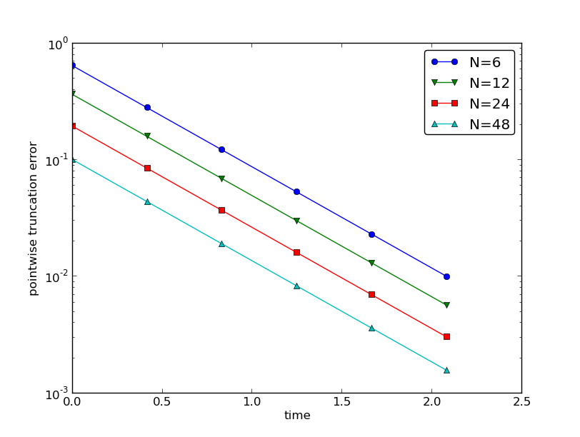
The task of this section is to demonstrate how we can compute the truncation error \(R\) numerically. For example, the truncation error of the Forward Euler scheme applied to the decay ODE \(u'=-ua\) is \[ R^n = [D_t^+u_{\text{e}} + au_{\text{e}}]^n \tp \tag{10.20}\] If we happen to know the exact solution \(u_{\text{e}}(t)\), we can easily evaluate \(R^n\) from the above formula.
To estimate how \(R\) varies with the discretization parameter \(\Delta
t\), which has been our focus in the previous mathematical derivations, we first make the assumption that \(R=C\Delta t^r\) for appropriate constants \(C\) and \(r\) and small enough \(\Delta t\). The rate \(r\) can be estimated from a series of experiments where \(\Delta t\) is varied. Suppose we have \(m\) experiments \((\Delta t_i, R_i)\), \(i=0,\ldots,m-1\). For two consecutive experiments \((\Delta t_{i-1}, R_{i-1})\) and \((\Delta t_i, R_i)\), a corresponding \(r_{i-1}\) can be estimated by \[
r_{i-1} = \frac{\ln (R_{i-1}/R_i)}{\ln (\Delta t_{i-1}/\Delta t_i)},
\tag{10.21}\] for \(i=1,\ldots,m-1\). Note that the truncation error \(R_i\) varies through the mesh, so (10.21) is to be applied pointwise. A complicating issue is that \(R_i\) and \(R_{i-1}\) refer to different meshes. Pointwise comparisons of the truncation error at a certain point in all meshes therefore requires any computed \(R\) to be restricted to the coarsest mesh and that all finer meshes contain all the points in the coarsest mesh. Suppose we have \(N_0\) intervals in the coarsest mesh. Inserting a superscript \(n\) in (10.21), where \(n\) counts mesh points in the coarsest mesh, \(n=0,\ldots,N_0\), leads to the formula \[
r_{i-1}^n = \frac{\ln (R_{i-1}^n/R_i^n)}{\ln (\Delta t_{i-1}/\Delta t_i)} \tp
\tag{10.22}\] Experiments are most conveniently defined by \(N_0\) and a number of refinements \(m\). Suppose each mesh has twice as many cells \(N_i\) as the previous one: \[
N_i = 2^iN_0,\quad \Delta t_i = TN_i^{-1},
\] where \([0,T]\) is the total time interval for the computations. Suppose the computed \(R_i\) values on the mesh with \(N_i\) intervals are stored in an array R[i] (R being a list of arrays, one for each mesh). Restricting this \(R_i\) function to the coarsest mesh means extracting every \(N_i/N_0\) point and is done as follows:
stride = N[i]/N_0
R[i] = R[i][::stride]
The quantity R[i][n] now corresponds to \(R_i^n\).
In addition to estimating \(r\) for the pointwise values of \(R=C\Delta t^r\), we may also consider an integrated quantity on mesh \(i\), \[ R_{I,i} = \left(\Delta t_i\sum_{n=0}^{N_i} (R_i^n)^2\right)^\half\approx \int_0^T R_i(t)dt \tp \] The sequence \(R_{I,i}\), \(i=0,\ldots,m-1\), is also expected to behave as \(C\Delta t^r\), with the same \(r\) as for the pointwise quantity \(R\), as \(\Delta t\rightarrow 0\).
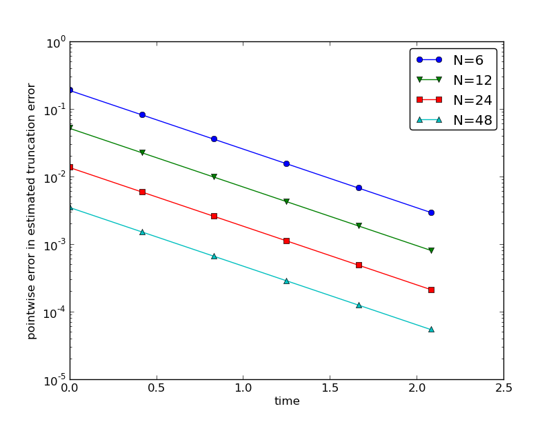
The function below computes the \(R_i\) and \(R_{I,i}\) quantities, plots them and compares with the theoretically derived truncation error (R_a) if available.
import numpy as np

def estimate(truncation_error, T, N_0, m, makeplot=True):
    """
    Compute the truncation error in a problem with one independent
    variable, using m meshes, and estimate the convergence
    rate of the truncation error.

    The user-supplied function truncation_error(dt, N) computes
    the truncation error on a uniform mesh with N intervals of
    length dt::

      R, t, R_a = truncation_error(dt, N)

    where R holds the truncation error at points in the array t,
    and R_a are the corresponding theoretical truncation error
    values (None if not available).

    The truncation_error function is run on a series of meshes
    with 2**i*N_0 intervals, i=0,1,...,m-1.
    The values of R and R_a are restricted to the coarsest mesh.
    and based on these data, the convergence rate of R (pointwise)
    and time-integrated R can be estimated empirically.
    """
    N = [2**i * N_0 for i in range(m)]

    R_I = np.zeros(m)  # time-integrated R values on various meshes
    R = [None] * m  # time series of R restricted to coarsest mesh
    R_a = [None] * m  # time series of R_a restricted to coarsest mesh
    dt = np.zeros(m)
    legends_R = []
    legends_R_a = []  # all legends of curves

    for i in range(m):
        dt[i] = T / float(N[i])
        R[i], t, R_a[i] = truncation_error(dt[i], N[i])

        R_I[i] = np.sqrt(dt[i] * np.sum(R[i] ** 2))

        if i == 0:
            t_coarse = t  # the coarsest mesh

        stride = N[i] / N_0
        R[i] = R[i][::stride]  # restrict to coarsest mesh
        R_a[i] = R_a[i][::stride]

        if makeplot:
            plt.figure(1)
            plt.plot(t_coarse, R[i])
            plt.yscale("log")
            legends_R.append("N=%d" % N[i])

            plt.figure(2)
            plt.plot(t_coarse, R_a[i] - R[i])
            plt.yscale("log")
            legends_R_a.append("N=%d" % N[i])

    if makeplot:
        plt.figure(1)
        plt.xlabel("time")
        plt.ylabel("pointwise truncation error")
        plt.legend(legends_R)
        plt.savefig("R_series.png")
        plt.savefig("R_series.pdf")
        plt.figure(2)
        plt.xlabel("time")
        plt.ylabel("pointwise error in estimated truncation error")
        plt.legend(legends_R_a)
        plt.savefig("R_error.png")
        plt.savefig("R_error.pdf")

    r_R_I = convergence_rates(dt, R_I)
    print("R integrated in time; r:", end=" ")
    print(" ".join(["%.1f" % r for r in r_R_I]))
    R = np.array(R)  # two-dim. numpy array
    r_R = [convergence_rates(dt, R[:, n])[-1] for n in range(len(t_coarse))]
The first makeplot block demonstrates how to build up two figures in parallel, using plt.figure(i) to create and switch to figure number i. Figure numbers start at 1. A logarithmic scale is used on the \(y\) axis since we expect that \(R\) as a function of time (or mesh points) is exponential. The reason is that the theoretical estimate (10.17) contains \(u_{\text{e}}''\), which for the present model goes like \(e^{-at}\). Taking the logarithm makes a straight line.
The code follows closely the previously stated mathematical formulas, but the statements for computing the convergence rates might deserve an explanation. The generic help function convergence_rate(h, E) computes and returns \(r_{i-1}\), \(i=1,\ldots,m-1\) from (10.22), given \(\Delta t_i\) in h and \(R_i^n\) in E:
def convergence_rates(h, E):
    from math import log
    r = [log(E[i]/E[i-1])/log(h[i]/h[i-1])
         for i in range(1, len(h))]
    return r
Calling r_R_I = convergence_rates(dt, R_I) computes the sequence of rates \(r_0,r_1,\ldots,r_{m-2}\) for the model \(R_I\sim\Delta t^r\), while the statements
R = np.array(R)  # two-dim. numpy array
r_R = [convergence_rates(dt, R[:,n])[-1]
       for n in range(len(t_coarse))]
compute the final rate \(r_{m-2}\) for \(R^n\sim\Delta t^r\) at each mesh point \(t_n\) in the coarsest mesh. This latter computation deserves more explanation. Since R[i][n] holds the estimated truncation error \(R_i^n\) on mesh \(i\), at point \(t_n\) in the coarsest mesh, R[:,n] picks out the sequence \(R_i^n\) for \(i=0,\ldots,m-1\). The convergence_rate function computes the rates at \(t_n\), and by indexing [-1] on the returned array from convergence_rate, we pick the rate \(r_{m-2}\), which we believe is the best estimation since it is based on the two finest meshes.
The estimate function is available in a module trunc_empir.py. Let us apply this function to estimate the truncation error of the Forward Euler scheme. We need a function decay_FE(dt, N) that can compute (10.20) at the points in a mesh with time step dt and N intervals:
import numpy as np
import trunc_empir

def decay_FE(dt, N):
    dt = float(dt)
    t = np.linspace(0, N * dt, N + 1)
    u_e = I * np.exp(-a * t)  # exact solution, I and a are global
    u = u_e  # naming convention when writing up the scheme
    R = np.zeros(N)

    for n in range(0, N):
        R[n] = (u[n + 1] - u[n]) / dt + a * u[n]

    R_a = 0.5 * I * (-a) ** 2 * np.exp(-a * t) * dt

    return R, t[:-1], R_a[:-1]

if __name__ == "__main__":
    I = 1
    a = 2  # global variables needed in decay_FE
    trunc_empir.estimate(decay_FE, T=2.5, N_0=6, m=4, makeplot=True)
The estimated rates for the integrated truncation error \(R_I\) become 1.1, 1.0, and 1.0 for this sequence of four meshes. All the rates for \(R^n\), computed as r_R, are also very close to 1 at all mesh points. The agreement between the theoretical formula (10.17) and the computed quantity (ref(10.20)) is very good, as illustrated in Figures Figure 10.1 and Figure 10.2. The program trunc_decay_FE.py was used to perform the simulations and it can easily be modified to test other schemes (see also Exercise Section 10.34).
10.15 Increasing the accuracy by adding correction terms
Now we ask the question: can we add terms in the differential equation that can help increase the order of the truncation error? To be precise, let us revisit the Forward Euler scheme for \(u'=-au\), insert the exact solution \(u_{\text{e}}\), include a residual \(R\), but also include new terms \(C\): \[ \lbrack D_t^+ u_{\text{e}} + au_{\text{e}} = C + R \rbrack^n\tp \tag{10.23}\] Inserting the Taylor expansions for \([D_t^+u_{\text{e}}]^n\) and keeping terms up to 3rd order in \(\Delta t\) gives the equation \[ \half u_{\text{e}}''(t_n)\Delta t - \frac{1}{6}u_{\text{e}}'''(t_n)\Delta t^2 + \frac{1}{24}u_{\text{e}}''''(t_n)\Delta t^3 + \Oof{\Delta t^4} = C^n + R^n\tp \] Can we find \(C^n\) such that \(R^n\) is \(\Oof{\Delta t^2}\)? Yes, by setting \[ C^n = \half u_{\text{e}}''(t_n)\Delta t, \] we manage to cancel the first-order term and \[ R^n = \frac{1}{6}u_{\text{e}}'''(t_n)\Delta t^2 + \Oof{\Delta t^3}\tp \] The correction term \(C^n\) introduces \(\half\Delta t u''\) in the discrete equation, and we have to get rid of the derivative \(u''\). One idea is to approximate \(u''\) by a second-order accurate finite difference formula, \(u''\approx (u^{n+1}-2u^n+u^{n-1})/\Delta t^2\), but this introduces an additional time level with \(u^{n-1}\). Another approach is to rewrite \(u''\) in terms of \(u'\) or \(u\) using the ODE: \[ u'=-au\quad\Rightarrow\quad u''=-au' = -a(-au)= a^2u\tp \] This means that we can simply set \(C^n = {\half}a^2\Delta t u^n\). We can then either solve the discrete equation \[ [D_t^+ u = -au + {\half}a^2\Delta t u]^n, \tag{10.24}\] or we can equivalently discretize the perturbed ODE \[ u' = -\hat au ,\quad \hat a = a(1 - {\half}a\Delta t), \tag{10.25}\] by a Forward Euler method. That is, we replace the original coefficient \(a\) by the perturbed coefficient \(\hat a\). Observe that \(\hat a\rightarrow a\) as \(\Delta t\rightarrow 0\).
The Forward Euler method applied to (10.25) results in \[ [D_t^+ u = -a(1 - {\half}a\Delta t)u]^n\tp \] We can control our computations and verify that the truncation error of the scheme above is indeed \(\Oof{\Delta t^2}\).
Another way of revealing the fact that the perturbed ODE leads to a more accurate solution is to look at the amplification factor. Our scheme can be written as \[ u^{n+1} = Au^n,\quad A = 1-\hat a\Delta t = 1 - p + {\half}p^2,\quad p=a\Delta t, \] The amplification factor \(A\) as a function of \(p=a\Delta t\) is seen to be the first three terms of the Taylor series for the exact amplification factor \(e^{-p}\). The Forward Euler scheme for \(u=-au\) gives only the first two terms \(1-p\) of the Taylor series for \(e^{-p}\). That is, using \(\hat a\) increases the order of the accuracy in the amplification factor.
Instead of replacing \(u''\) by \(a^2u\), we use the relation \(u''=-au'\) and add a term \(-{\half}a\Delta t u'\) in the ODE: \[ u'=-au - {\half}a\Delta t u'\quad\Rightarrow\quad \left( 1 + {\half}a\Delta t\right) u' = -au\tp \] Using a Forward Euler method results in \[ \left( 1 + {\half}a\Delta t\right)\frac{u^{n+1}-u^n}{\Delta t} = -au^n, \] which after some algebra can be written as \[ u^{n+1} = \frac{1 - {\half}a\Delta t}{1+{\half}a\Delta t}u^n\tp \] This is the same formula as the one arising from a Crank-Nicolson scheme applied to \(u'=-au\)! It is now recommended to do Exercise Section 10.35 and repeat the above steps to see what kind of correction term is needed in the Backward Euler scheme to make it second order.
The Crank-Nicolson scheme is a bit more challenging to analyze, but the ideas and techniques are the same. The discrete equation reads \[ [D_t u = -au ]^{n+\half}, \] and the truncation error is defined through \[ [D_t u_{\text{e}} + a\overline{u_{\text{e}}}^{t} = C + R]^{n+\half}, \] where we have added a correction term. We need to Taylor expand both the discrete derivative and the arithmetic mean with aid of 10.9 and 10.11, respectively. The result is \[ \frac{1}{24}u_{\text{e}}'''(t_{n+\half})\Delta t^2 + \Oof{\Delta t^4} + \frac{a}{8}u_{\text{e}}''(t_{n+\half})\Delta t^2 + \Oof{\Delta t^4} = C^{n+\half} + R^{n+\half}\tp \] The goal now is to make \(C^{n+\half}\) cancel the \(\Delta t^2\) terms: \[ C^{n+\half} = \frac{1}{24}u_{\text{e}}'''(t_{n+\half})\Delta t^2 + \frac{a}{8}u_{\text{e}}''(t_{n})\Delta t^2\tp \] Using \(u'=-au\), we have that \(u''=a^2u\), and we find that \(u'''=-a^3u\). We can therefore solve the perturbed ODE problem \[ u' = -\hat a u,\quad \hat a = a(1 - \frac{1}{12}a^2\Delta t^2), \] by the Crank-Nicolson scheme and obtain a method that is of fourth order in \(\Delta t\). Exercise Section 10.36 encourages you to implement these correction terms and calculate empirical convergence rates to verify that higher-order accuracy is indeed obtained in real computations.
10.16 Extension to variable coefficients
Let us address the decay ODE with variable coefficients, \[ u'(t) = -a(t)u(t) + b(t), \] discretized by the Forward Euler scheme, \[ [D_t^+ u = -au + b]^n \tp \] The truncation error \(R\) is as always found by inserting the exact solution \(u_{\text{e}}(t)\) in the discrete scheme: \[ [D_t^+ u_{\text{e}} + au_{\text{e}} - b = R]^n \tp \] Using 10.6, \[ u_{\text{e}}'(t_n) - \half u_{\text{e}}''(t_n)\Delta t + \Oof{\Delta t^2} + a(t_n)u_{\text{e}}(t_n) - b(t_n) = R^n \tp \] Because of the ODE, \[ u_{\text{e}}'(t_n) + a(t_n)u_{\text{e}}(t_n) - b(t_n) =0, \] we are left with the result \[ R^n = -\half u_{\text{e}}''(t_n)\Delta t + \Oof{\Delta t^2} \tp \tag{10.26}\] We see that the variable coefficients do not pose any additional difficulties in this case. Exercise Section 10.37 takes the analysis above one step further to the Crank-Nicolson scheme.
10.17 Exact solutions of the finite difference equations
Having a mathematical expression for the numerical solution is very valuable in program verification, since we then know the exact numbers that the program should produce. Looking at the various formulas for the truncation errors in 10.9 and 10.13 in Section Section 10.7, we see that all but two of the \(R\) expressions contain a second or higher order derivative of \(u_{\text{e}}\). The exceptions are the geometric and harmonic means where the truncation error involves \(u_{\text{e}}'\) and even \(u_{\text{e}}\) in case of the harmonic mean. So, apart from these two means, choosing \(u_{\text{e}}\) to be a linear function of \(t\), \(u_{\text{e}} = ct+d\) for constants \(c\) and \(d\), will make the truncation error vanish since \(u_{\text{e}}''=0\). Consequently, the truncation error of a finite difference scheme will be zero since the various approximations used will all be exact. This means that the linear solution is an exact solution of the discrete equations.
In a particular differential equation problem, the reasoning above can be used to determine if we expect a linear \(u_{\text{e}}\) to fulfill the discrete equations. To actually prove that this is true, we can either compute the truncation error and see that it vanishes, or we can simply insert \(u_{\text{e}}(t)=ct+d\) in the scheme and see that it fulfills the equations. The latter method is usually the simplest. It will often be necessary to add some source term to the ODE in order to allow a linear solution.
Many ODEs are discretized by centered differences. From Section Section 10.7 we see that all the centered difference formulas have truncation errors involving \(u_{\text{e}}'''\) or higher-order derivatives. A quadratic solution, e.g., \(u_{\text{e}}(t) =t^2 + ct + d\), will then make the truncation errors vanish. This observation can be used to test if a quadratic solution will fulfill the discrete equations. Note that a quadratic solution will not obey the equations for a Crank-Nicolson scheme for \(u'=-au+b\) because the approximation applies an arithmetic mean, which involves a truncation error with \(u_{\text{e}}''\).
10.18 Computing truncation errors in nonlinear problems
The general nonlinear ODE \[ u'=f(u,t), \tag{10.27}\] can be solved by a Crank-Nicolson scheme \[ [D_t u=\overline{f}^{t}]^{n+\half}\tp \tag{10.28}\] The truncation error is as always defined as the residual arising when inserting the exact solution \(u_{\text{e}}\) in the scheme: \[ [D_t u_{\text{e}} - \overline{f}^{t}= R]^{n+\half}\tp \tag{10.29}\] Using 10.11 for \(\overline{f}^{t}\) results in
\[\begin{align*} [\overline{f}^{t}]^{n+\half} &= \half(f(u_{\text{e}}^n,t_n) + f(u_{\text{e}}^{n+1},t_{n+1}))\\ &= f(u_{\text{e}}^{n+\half},t_{n+\half}) + \frac{1}{8}u_{\text{e}}''(t_{n+\half})\Delta t^2 + \Oof{\Delta t^4}\tp \end{align*}\] With 10.9 the discrete equations (10.29) lead to \[ u_{\text{e}}'(t_{n+\half}) + \frac{1}{24}u_{\text{e}}'''(t_{n+\half})\Delta t^2 + f(u_{\text{e}}^{n+\half},t_{n+\half}) - \frac{1}{8}u_{\text{e}}''(t_{n+\half})\Delta t^2 + \Oof{\Delta t^4} = R^{n+\half}\tp \] Since \(u_{\text{e}}'(t_{n+\half}) - f(u_{\text{e}}^{n+\half},t_{n+\half})=0\), the truncation error becomes \[ R^{n+\half} = (\frac{1}{24}u_{\text{e}}'''(t_{n+\half}) + \frac{1}{8}u_{\text{e}}''(t_{n+\half})) \Delta t^2\tp \] The computational techniques worked well even for this nonlinear ODE.
10.19 Linear model without damping
The next example on computing the truncation error involves the following ODE for vibration problems: \[ u''(t) + \omega^2 u(t) = 0\tp \tag{10.30}\] Here, \(\omega\) is a given constant.
10.19.1 The truncation error of a centered finite difference scheme
Using a standard, second-ordered, central difference for the second-order derivative in time, we have the scheme \[ [D_tD_t u + \omega^2u=0]^n \tp \tag{10.31}\]
Inserting the exact solution \(u_{\text{e}}\) in this equation and adding a residual \(R\) so that \(u_{\text{e}}\) can fulfill the equation results in \[ [D_tD_t u_{\text{e}} + \omega^2u_{\text{e}} =R]^n \tp \] To calculate the truncation error \(R^n\), we use 10.4, i.e., \[ [D_tD_t u_{\text{e}}]^n = u_{\text{e}}''(t_n) + \frac{1}{12}u_{\text{e}}''''(t_n)\Delta t^2 + \Oof{\Delta t^4}, \] and the fact that \(u_{\text{e}}''(t) + \omega^2u_{\text{e}}(t)=0\). The result is \[ R^n = \frac{1}{12}u_{\text{e}}''''(t_n)\Delta t^2 + \Oof{\Delta t^4} \tp \] ### The truncation error of approximating \(u'(0)\) The initial conditions for (10.30) are \(u(0)=I\) and \(u'(0)=V\). The latter involves a finite difference approximation. The standard choice \[ [D_{2t}u=V]^0, \] where \(u^{-1}\) is eliminated with the aid of the discretized ODE for \(n=0\), involves a centered difference with an \(\Oof{\Delta t^2}\) truncation error given by 10.3. The simpler choice \[ [D_t^+u = V]^0, \] is based on a forward difference with a truncation error \(\Oof{\Delta t}\). A central question is if this initial error will impact the order of the scheme throughout the simulation. Exercise Section 10.40 asks you to perform an experiment to investigate this question.
10.19.2 Truncation error of the equation for the first step
We have shown that the truncation error of the difference used to approximate the initial condition \(u'(0)=0\) is \(\Oof{\Delta t^2}\), but we can also investigate the difference equation used for the first step. In a truncation error setting, the right way to view this equation is not to use the initial condition \([D_{2t}u=V]^0\) to express \(u^{-1}=u^1 - 2\Delta t V\) in order to eliminate \(u^{-1}\) from the discretized differential equation, but the other way around: the fundamental equation is the discretized initial condition \([D_{2t}u=V]^0\) and we use the discretized ODE \([D_tD_t + \omega^2 u=0]^0\) to eliminate \(u^{-1}\) in the discretized initial condition. From \([D_tD_t + \omega^2 u=0]^0\) we have \[ u^{-1} = 2u^0 - u^1 - \Delta t^2\omega^2 u^0, \] which inserted in \([D_{2t}u = V]^0\) gives \[ \frac{u^1 - u^0}{\Delta t} + \half\omega^2\Delta t u^0 = V\tp \tag{10.32}\] The first term can be recognized as a forward difference such that the equation can be written in operator notation as \[ [D_t^+ u + \half\omega^2\Delta t u = V]^0\tp \] The truncation error is defined as \[ [D_t^+ u_{\text{e}} + \half\omega^2\Delta t u_{\text{e}} - V = R]^0\tp \] Using 10.6 with one more term in the Taylor series, we get that \[ u_{\text{e}}'(0) + \half u_{\text{e}}''(0)\Delta t + \frac{1}{6}u_{\text{e}}'''(0)\Delta t^2 + \Oof{\Delta t^3} + \half\omega^2\Delta t u_{\text{e}}(0) - V = R^n\tp \] Now, \(u_{\text{e}}'(0)=V\) and \(u_{\text{e}}''(0)=-\omega^2 u_{\text{e}}(0)\) so we get \[ R^n = \frac{1}{6}u_{\text{e}}'''(0)\Delta t^2 + \Oof{\Delta t^3}\tp \] There is another way of analyzing the discrete initial condition, because eliminating \(u^{-1}\) via the discretized ODE can be expressed as \[ [ D_{2t} u + \Delta t(D_tD_t u - \omega^2 u) = V]^0\tp \tag{10.33}\] Writing out (10.33) shows that the equation is equivalent to (10.32). The truncation error is defined by \[ [ D_{2t} u_{\text{e}} + \Delta t(D_tD_t u_{\text{e}} - \omega^2 u_{\text{e}}) = V + R]^0\tp \] Replacing the difference via 10.3 and 10.4, as well as using \(u_{\text{e}}'(0)=V\) and \(u_{\text{e}}''(0) = -\omega^2u_{\text{e}}(0)\), gives \[ R^n = \frac{1}{6}u_{\text{e}}'''(0)\Delta t^2 + \Oof{\Delta t^3}\tp \] ### Computing correction terms The idea of using correction terms to increase the order of \(R^n\) can be applied as described in Section Section 10.15. We look at \[ [D_tD_t u_{\text{e}} + \omega^2u_{\text{e}} =C + R]^n, \] and observe that \(C^n\) must be chosen to cancel the \(\Delta t^2\) term in \(R^n\). That is, \[ C^n = \frac{1}{12}u_{\text{e}}''''(t_n)\Delta t^2\tp \] To get rid of the 4th-order derivative we can use the differential equation: \(u''=-\omega^2u\), which implies \(u'''' = \omega^4 u\). Adding the correction term to the ODE results in \[ u'' + \omega^2(1 - \frac{1}{12}\omega^2\Delta t^2)u = 0\tp \tag{10.34}\] Solving this equation by the standard scheme \[ [D_tD_t u + \omega^2(1 - \frac{1}{12}\omega^2\Delta t^2)u=0]^n, \] will result in a scheme with truncation error \(\Oof{\Delta t^4}\).
We can use another set of arguments to justify that (10.34) leads to a higher-order method. Mathematical analysis of the scheme (10.31) reveals that the numerical frequency \(\tilde\omega\) is (approximately as \(\Delta t\rightarrow 0\)) \[
\tilde\omega = \omega (1+\frac{1}{24}\omega^2\Delta t^2)\tp
\] One can therefore attempt to replace \(\omega\) in the ODE by a slightly smaller \(\omega\) since the numerics will make it larger: \[
[ u'' + (\omega(1 - \frac{1}{24}\omega^2\Delta t^2))^2 u ]^n = 0\tp
\] Expanding the squared term and omitting the higher-order term \(\Delta t^4\) gives exactly the ODE (10.34). Experiments show that \(u^n\) is computed to 4th order in \(\Delta t\). You can confirm this by running a little program in the vib directory:
from vib_undamped import convergence_rates, solver_adjust_w

r = convergence_rates(
      m=5, solver_function=solver_adjust_w, num_periods=8)
One will see that the rates r lie around 4.
10.20 Model with damping and nonlinearity
The model (10.30) can be extended to include damping \(\beta u'\), a nonlinear restoring (spring) force \(s(u)\), and some known excitation force \(F(t)\): \[ mu'' + \beta u' + s(u) =F(t)\tp \tag{10.35}\] The coefficient \(m\) usually represents the mass of the system. This governing equation can be discretized by centered differences: \[ [mD_tD_t u + \beta D_{2t} u + s(u)=F]^n \tp \] The exact solution \(u_{\text{e}}\) fulfills the discrete equations with a residual term: \[ [mD_tD_t u_{\text{e}} + \beta D_{2t} u_{\text{e}} + s(u_{\text{e}})=F + R]^n \tp \] Using 10.4 and 10.3 we get
\[\begin{align*} \lbrack mD_tD_t u_{\text{e}} + \beta D_{2t} u_{\text{e}}\rbrack^n &= mu_{\text{e}}''(t_n) + \beta u_{\text{e}}'(t_n) + \\ &\quad \left(\frac{m}{12}u_{\text{e}}''''(t_n) + \frac{\beta}{6}u_{\text{e}}'''(t_n)\right)\Delta t^2 + \Oof{\Delta t^4} \end{align*}\] Combining this with the previous equation, we can collect the terms \[ mu_{\text{e}}''(t_n) + \beta u_{\text{e}}'(t_n) + \omega^2u_{\text{e}}(t_n) + s(u_{\text{e}}(t_n)) - F^n, \] and set this sum to zero because \(u_{\text{e}}\) solves the differential equation. We are left with the truncation error \[ R^n = \left(\frac{m}{12}u_{\text{e}}''''(t_n) + \frac{\beta}{6}u_{\text{e}}'''(t_n)\right)\Delta t^2 + \Oof{\Delta t^4}, \tag{10.36}\] so the scheme is of second order.
According to (10.36), we can add correction terms \[ C^n = \left(\frac{m}{12}u_{\text{e}}''''(t_n) + \frac{\beta}{6}u_{\text{e}}'''(t_n)\right)\Delta t^2, \] to the right-hand side of the ODE to obtain a fourth-order scheme. However, expressing \(u''''\) and \(u'''\) in terms of lower-order derivatives is now harder because the differential equation is more complicated:
\[\begin{align*} u''' &= \frac{1}{m}(F' - \beta u'' - s'(u)u'),\\ u'''' &= \frac{1}{m}(F'' - \beta u''' - s''(u)(u')^2 - s'(u)u''),\\ &= \frac{1}{m}(F'' - \beta \frac{1}{m}(F' - \beta u'' - s'(u)u') - s''(u)(u')^2 - s'(u)u'')\tp \end{align*}\] It is not impossible to discretize the resulting modified ODE, but it is up to debate whether correction terms are feasible and the way to go. Computing with a smaller \(\Delta t\) is usually always possible in these problems to achieve the desired accuracy.
10.21 Extension to quadratic damping
Instead of the linear damping term \(\beta u'\) in (10.35) we now consider quadratic damping \(\beta |u'|u'\): \[ mu'' + \beta |u'|u' + s(u) =F(t)\tp \tag{10.37}\] A centered difference for \(u'\) gives rise to a nonlinearity, which can be linearized using a geometric mean: \([|u'|u']^n \approx |[u']^{n-\half}|[u']^{n+\half}\). The resulting scheme becomes \[ [mD_t D_t u]^n + \beta |[D_{t} u]^{n-\half}|[D_t u]^{n+\half} + s(u^n)=F^n\tp \] The truncation error is defined through \[ [mD_t D_t u_{\text{e}}]^n + \beta |[D_{t} u_{\text{e}}]^{n-\half}|[D_t u_{\text{e}}]^{n+\half} + s(u_{\text{e}}^n)-F^n = R^n\tp \] We start with expressing the truncation error of the geometric mean. According to 10.12,
\[\begin{align*} |[D_{t} u_{\text{e}}]^{n-\half}|[D_t u_{\text{e}}]^{n+\half} &= [|D_tu_{\text{e}}|D_tu_{\text{e}}]^n - \frac{1}{4}u_{\text{e}}'(t_n)^2\Delta t^2 +\\ &\quad \frac{1}{4}u_{\text{e}}(t_n)u_{\text{e}}''(t_n)\Delta t^2 + \Oof{\Delta t^4}\tp \end{align*}\] Using 10.9 for the \(D_tu_{\text{e}}\) factors results in \[ [|D_tu_{\text{e}}|D_tu_{\text{e}}]^n = |u_{\text{e}}' + \frac{1}{24}u_{\text{e}}'''(t_n)\Delta t^2 + \Oof{\Delta t^4}|(u_{\text{e}}' + \frac{1}{24}u_{\text{e}}'''(t_n)\Delta t^2 + \Oof{\Delta t^4}) \] We can remove the absolute value since it essentially gives a factor 1 or -1 only. Calculating the product, we have the leading-order terms \[ [D_tu_{\text{e}} D_tu_{\text{e}}]^n = (u_{\text{e}}'(t_n))^2 + \frac{1}{12}u_{\text{e}}(t_n)u_{\text{e}}'''(t_n)\Delta t^2 + \Oof{\Delta t^4}\tp \] With \[ m[D_t D_tu_{\text{e}}]^n = mu_{\text{e}}''(t_n) + \frac{m}{12}u_{\text{e}}''''(t_n)\Delta t^2 +\Oof{\Delta t^4}, \] and using the differential equation on the form \(mu'' + \beta (u')^2 + s(u)=F\), we end up with \[ R^n = (\frac{m}{12}u_{\text{e}}''''(t_n) + \frac{\beta}{12}u_{\text{e}}(t_n)u_{\text{e}}'''(t_n)) \Delta t^2 + \Oof{\Delta t^4}\tp \] This result demonstrates that we have second-order accuracy also with quadratic damping. The key elements that lead to the second-order accuracy is that the difference approximations are \(\Oof{\Delta t^2}\) and the geometric mean approximation is also \(\Oof{\Delta t^2}\).
10.22 The general model formulated as first-order ODEs
The second-order model (10.37) can be formulated as a first-order system,
\[ v' = \frac{1}{m}\left( F(t) - \beta |v|v - s(u)\right), \tag{10.38}\] \[ u' = v\tp \tag{10.39}\] The system (10.38)-(10.39) can be solved either by a forward-backward scheme (the Euler-Cromer method) or a centered scheme on a staggered mesh.
10.22.1 The Euler-Cromer scheme
The discretization is based on the idea of stepping (10.38) forward in time and then using a backward difference in (10.39) with the recently computed \(v^{n+1}\):
\[ \lbrack D_t^+v = \frac{1}{m}( F(t) - \beta |v|v - s(u)) \rbrack^{n+1}\tp \tag{10.40}\] \[ \lbrack D_t^- u = v \rbrack^{n+1}, \tag{10.41}\] For a truncation error analysis, we rewrite the system in vector-matrix form. Consider the linear case without damping, \[ v^{n+1} = v^n -\Delta t\omega^2u^n,\quad u^{n+1} = u^n + \Delta t v^{n+1}\tp \] We introduce the vector \(w=(v,u)\) and write the system as \[ Aw^{n+1} = Bw^n, \quad A = \left\lbrack\begin{array}{ll} 1 & 0\\ 1 & -\Delta t\end{array}\right\rbrack, \quad B = \left\lbrack\begin{array}{ll} 1 & -\Delta t\omega^2\\ 0 & 1\end{array}\right\rbrack\tp \] The exact solution \(w_{\text{e}}\) satisfies \[ Aw_{\text{e}}^{n+1} = Bw^n + \Delta t R^n, \] where \(R^n\) is the residual, which has to be multiplied by \(\Delta t\) since we have already done that in the discrete equation.
The corresponding differential equation in \(w\) becomes \[ \frac{dw}{dt} = Cw,\quad C = \left\lbrack\begin{array}{ll} 0 & -\omega^2\\ 1 & 0\end{array}\right\rbrack\tp \] We realize that \(d^2w = C^2 w\), and in general \(d^mw=C^w\). Using these formulas to get rid of the derivatives in a Taylor expansion of \(w_{\text{e}}^{n+1}\) around \(t_n\) gives \[ A(w_{\text{e}}^n + \Delta t Cw_{\text{e}}^n + \half \Delta t^2 C^2 w_{\text{e}}^n + \cdots) = Bw_{\text{e}}^n + \Delta t R^n\tp \] From this we get
\[\begin{align*} R^n &= \frac{1}{\Delta t}(A - B + \Delta t AC + \half\Delta t^2 AC^2 +\cdots)w_{\text{e}}^n\\ &\sim \mathcal(1) \end{align*}\] This does not work out…
Each ODE will have a truncation error when inserting the exact solutions \(u_{\text{e}}\) and \(v_{\text{e}}\) in (10.40)-(10.41):
\[ \lbrack D_t^+ u_{\text{e}} = v_{\text{e}} + R_u \rbrack^n, \tag{10.42}\] \[ \lbrack D_t^-v_{\text{e}} \rbrack^{n+1} = \frac{1}{m}( F(t_{n+1}) - \beta |v_{\text{e}}(t_n)|v_{\text{e}}(t_{n+1}) - s(u_{\text{e}}(t_{n+1}))) + R_v^{n+1}\tp \tag{10.43}\] Application of 10.6 and 10.5 in (10.42) and (10.43), respectively, gives
\[ u_{\text{e}}'(t_n) + \half u_{\text{e}}''(t_n)\Delta t + \Oof{\Delta t^2} = v_{\text{e}}(t_n) + R_u^n, \tag{10.44}\] \[ \begin{split} v_{\text{e}}'(t_{n+1}) - \half v_{\text{e}}''(t_{n+1})\Delta t + \Oof{\Delta t^2} &= \frac{1}{m}(F(t_{n+1}) - \beta|v_{\text{e}}(t_n)|v_{\text{e}}(t_{n+1}) +\\ &\quad s(u_{\text{e}}(t_{n+1}))+ R_v^n\tp \end{split} \tag{10.45}\] Since \(u_{\text{e}} ' = v_{\text{e}}\), (10.44) gives \[ R_u^n = \half u_{\text{e}}''(t_n)\Delta t + \Oof{\Delta t^2}\tp \] In (10.45) we can collect the terms that constitute the ODE, but the damping term has the wrong form. Let us drop the absolute value in the damping term for simplicity. Adding a subtracting the right form \(v^{n+1}v^{n+1}\) helps:
\[\begin{align*} v_{\text{e}}'(t_{n+1}) &- \frac{1}{m}(F(t_{n+1}) - \beta v_{\text{e}}(t_{n+1})v_{\text{e}}(t_{n+1}) + s(u_{\text{e}}(t_{n+1})) + \\ & (\beta v_{\text{e}}(t_n)v_{\text{e}}(t_{n+1}) - \beta v_{\text{e}}(t_{n+1})v_{\text{e}}(t_{n+1}))), \end{align*}\] which reduces to
\[\begin{align*} \frac{\beta}{m}v_{\text{e}}(t_{n+1}(v_{\text{e}}(t_n) - v_{\text{e}}(t_{n+1})) &= \frac{\beta}{m}v_{\text{e}}(t_{n+1}[D_t^-v_{\text{e}}]^{n+1}\Delta t\\ &= \frac{\beta}{m}v_{\text{e}}(t_{n+1}(v_{\text{e}}'(t_{n+1})\Delta t + -\half v_{\text{e}}'''(t_{n+1})\Delta t^ + \Oof{\Delta t^3})\tp \end{align*}\] We end with \(R_u^n\) and \(R_v^{n+1}\) as \(\Oof{\Delta t}\), simply because all the building blocks in the schemes (the forward and backward differences and the linearization trick) are only first-order accurate. However, this analysis is misleading: the building blocks play together in a way that makes the scheme second-order accurate. This is shown by considering an alternative, yet equivalent, formulation of the above scheme.
10.22.2 A centered scheme on a staggered mesh
We now introduce a staggered mesh where we seek \(u\) at mesh points \(t_n\) and \(v\) at points \(t_{n+\half}\) in between the \(u\) points. The staggered mesh makes it easy to formulate centered differences in the system (10.38)-(10.39):
\[ \lbrack D_t u = v \rbrack^{n-\half}, \] \[ \lbrack D_t v = \frac{1}{m}( F(t) - \beta |v|v - s(u)) \rbrack^{n}\tp \tag{10.46}\] The term \(|v^n|v^n\) causes trouble since \(v^n\) is not computed, only \(v^{n-\half}\) and \(v^{n+\half}\). Using geometric mean, we can express \(|v^n|v^n\) in terms of known quantities: \(|v^n|v^n \approx |v^{n-\half}|v^{n+\half}\). We then have
\[ \lbrack D_t u \rbrack^{n-\half} = v^{n-\half}, \] \[ \lbrack D_t v \rbrack^n = \frac{1}{m}( F(t_n) - \beta |v^{n-\half}|v^{n+\half} - s(u^n))\tp \tag{10.47}\] The truncation error in each equation fulfills
\[\begin{align*} \lbrack D_t u_{\text{e}} \rbrack^{n-\half} &= v_{\text{e}}(t_{n-\half}) + R_u^{n-\half},\\ \lbrack D_t v_{\text{e}} \rbrack^n &= \frac{1}{m}( F(t_n) - \beta |v_{\text{e}}(t_{n-\half})|v_{\text{e}}(t_{n+\half}) - s(u^n)) + R_v^n\tp \end{align*}\] The truncation error of the centered differences is given by 10.9, and the geometric mean approximation analysis can be taken from 10.12. These results lead to \[ u_{\text{e}}'(t_{n-\half}) + \frac{1}{24}u_{\text{e}}'''(t_{n-\half})\Delta t^2 + \Oof{\Delta t^4} = v_{\text{e}}(t_{n-\half}) + R_u^{n-\half}, \] and \[ v_{\text{e}}'(t_n) = \frac{1}{m}( F(t_n) - \beta |v_{\text{e}}(t_n)|v_{\text{e}}(t_n) + \Oof{\Delta t^2} - s(u^n)) + R_v^n\tp \] The ODEs fulfilled by \(u_{\text{e}}\) and \(v_{\text{e}}\) are evident in these equations, and we achieve second-order accuracy for the truncation error in both equations: \[ R_u^{n-\half}= \Oof{\Delta t^2}, \quad R_v^n = \Oof{\Delta t^2}\tp \]
10.23 Linear wave equation in 1D
The standard, linear wave equation in 1D for a function \(u(x,t)\) reads \[ \frac{\partial^2 u}{\partial t^2} = c^2\frac{\partial^2 u}{\partial x^2} + f(x,t),\quad x\in (0, L),\ t\in (0,T], \tag{10.48}\] where \(c\) is the constant wave velocity of the physical medium in \([0,L]\). The equation can also be more compactly written as \[ u_{tt} = c^2u_{xx} + f,\quad x\in (0, L),\ t\in (0,T], \tag{10.49}\] Centered, second-order finite differences are a natural choice for discretizing the derivatives, leading to \[ [D_t D_t u = c^2 D_xD_x u + f]^n_i \tp \tag{10.50}\]
Inserting the exact solution \(u_{\text{e}}(x,t)\) in (10.50) makes this function fulfill the equation if we add the term \(R\): \[ [D_t D_t u_{\text{e}} = c^2 D_xD_x u_{\text{e}} + f + R]^n_i \tag{10.51}\]
Our purpose is to calculate the truncation error \(R\). From 10.4 we have that \[ [D_t D_tu_{\text{e}}]_i^n = u_{\text{e},tt}(x_i,t_n) + \frac{1}{12}u_{\text{e},tttt}(x_i,t_n)\Delta t^2 + \Oof{\Delta t^4}, \] when we use a notation taking into account that \(u_{\text{e}}\) is a function of two variables and that derivatives must be partial derivatives. The notation \(u_{\text{e},tt}\) means \(\partial^2u_{\text{e}} /\partial t^2\).
The same formula may also be applied to the \(x\)-derivative term: \[ [D_xD_xu_{\text{e}}]_i^n = u_{\text{e},xx}(x_i,t_n) + \frac{1}{12}u_{\text{e},xxxx}(x_i,t_n)\Delta x^2 + \Oof{\Delta x^4}, \] Equation (10.51) now becomes
\[\begin{align*} u_{\text{e},tt} + \frac{1}{12}u_{\text{e},tttt}(x_i,t_n)\Delta t^2 &= c^2u_{\text{e},xx} + c^2\frac{1}{12}u_{\text{e},xxxx}(x_i,t_n)\Delta x^2 + f(x_i,t_n) + \\ & \quad \Oof{\Delta t^4,\Delta x^4} + R^n_i \end{align*}\] Because \(u_{\text{e}}\) fulfills the partial differential equation (PDE) (10.49), the first, third, and fifth term cancel out, and we are left with \[ R^n_i = \frac{1}{12}u_{\text{e},tttt}(x_i,t_n)\Delta t^2 - c^2\frac{1}{12}u_{\text{e},xxxx}(x_i,t_n)\Delta x^2 + \Oof{\Delta t^4,\Delta x^4}, \tag{10.52}\] showing that the scheme (10.50) is of second order in the time and space mesh spacing.
10.24 Finding correction terms
Can we add correction terms to the PDE and increase the order of \(R^n_i\) in (10.52)? The starting point is \[ [D_t D_t u_{\text{e}} = c^2 D_xD_x u_{\text{e}} + f + C + R]^n_i \tag{10.53}\] From the previous analysis we simply get (10.52) again, but now with \(C\): \[ R^n_i + C_i^n = \frac{1}{12}u_{\text{e},tttt}(x_i,t_n)\Delta t^2 - c^2\frac{1}{12}u_{\text{e},xxxx}(x_i,t_n)\Delta x^2 + \Oof{\Delta t^4,\Delta x^4}\tp \tag{10.54}\] The idea is to let \(C_i^n\) cancel the \(\Delta t^2\) and \(\Delta x^2\) terms to make \(R^n_i = \Oof{\Delta t^4,\Delta x^4}\): \[ C_i^n = \frac{1}{12}u_{\text{e},tttt}(x_i,t_n)\Delta t^2 - c^2\frac{1}{12}u_{\text{e},xxxx}(x_i,t_n)\Delta x^2\tp \] Essentially, it means that we add a new term \[ C = \frac{1}{12}\left( u_{tttt}\Delta t^2 - c^2u_{xxxx}\Delta x^2\right), \] to the right-hand side of the PDE. We must either discretize these 4th-order derivatives directly or rewrite them in terms of lower-order derivatives with the aid of the PDE. The latter approach is more feasible. From the PDE we have the operator equality \[ \frac{\partial^2}{\partial t^2} = c^2\frac{\partial^2}{\partial x^2}, \] so \[ u_{tttt} = c^2u_{xxtt},\quad u_{xxxx} = c^{-2}u_{ttxx}\tp \] Assuming \(u\) is smooth enough, so that \(u_{xxtt}=u_{ttxx}\), these relations lead to \[ C = \frac{1}{12}((c^2\Delta t^2 - \Delta x^2)u_{xx})_{tt}\tp \] A natural discretization is \[ C^n_i = \frac{1}{12}((c^2\Delta t^2 - \Delta x^2) [D_xD_xD_tD_t u]^n_i\tp \] Writing out \([D_xD_xD_tD_t u]^n_i\) as \([D_xD_x (D_tD_t u)]^n_i\) gives
\[\begin{align*} \frac{1}{\Delta t^2}\biggl( &\frac{u^{n+1}_{i+1} - 2u^{n}_{i+1} + u^{n-1}_{i+1}}{\Delta x^2} -2\\ &\frac{u^{n+1}_{i} - 2u^{n}_{i} + u^{n-1}_{i}}{\Delta x^2} + &\frac{u^{n+1}_{i-1} - 2u^{n}_{i-1} + u^{n-1}_{i-1}}{\Delta x^2} \biggr) \end{align*}\] Now the unknown values \(u^{n+1}_{i+1}\), \(u^{n+1}_{i}\), and \(u^{n+1}_{i-1}\) are coupled, and we must solve a tridiagonal system to find them. This is in principle straightforward, but it results in an implicit finite difference scheme, while we had a convenient explicit scheme without the correction terms.
10.25 Extension to variable coefficients
Now we address the variable coefficient version of the linear 1D wave equation, \[ \frac{\partial^2 u}{\partial t^2} = \frac{\partial}{\partial x} \left( \lambda(x)\frac{\partial u}{\partial x}\right), \] or written more compactly as \[ u_{tt} = (\lambda u_x)_x\tp \tag{10.55}\] The discrete counterpart to this equation, using arithmetic mean for \(\lambda\) and centered differences, reads \[ [D_t D_t u = D_x \overline{\lambda}^{x}D_x u]^n_i\tp \tag{10.56}\] The truncation error is the residual \(R\) in the equation \[ [D_t D_t u_{\text{e}} = D_x \overline{\lambda}^{x}D_x u_{\text{e}} + R]^n_i\tp \tag{10.57}\] The difficulty with (10.57) is how to compute the truncation error of the term \([D_x \overline{\lambda}^{x}D_x u_{\text{e}}]^n_i\).
We start by writing out the outer operator: \[ [D_x \overline{\lambda}^{x}D_x u_{\text{e}}]^n_i = \frac{1}{\Delta x}\left( [\overline{\lambda}^{x}D_x u_{\text{e}}]^n_{i+\half} - [\overline{\lambda}^{x}D_x u_{\text{e}}]^n_{i-\half} \right). \tag{10.58}\] With the aid of 10.9 and 10.11 we have
\[\begin{align*} \lbrack D_x u_{\text{e}} \rbrack^n_{i+\half} & = u_{\text{e},x}(x_{i+\half},t_n) + \frac{1}{24}u_{\text{e},xxx}(x_{i+\half},t_n)\Delta x^2 + \Oof{\Delta x^4},\\ \lbrack\overline{\lambda}^{x}\rbrack_{i+\half} &= \lambda(x_{i+\half}) + \frac{1}{8}\lambda''(x_{i+\half})\Delta x^2 + \Oof{\Delta x^4},\\ [\overline{\lambda}^{x}D_x u_{\text{e}}]^n_{i+\half} &= (\lambda(x_{i+\half}) + \frac{1}{8}\lambda''(x_{i+\half})\Delta x^2 + \Oof{\Delta x^4})\times\\ &\quad (u_{\text{e},x}(x_{i+\half},t_n) + \frac{1}{24}u_{\text{e},xxx}(x_{i+\half},t_n)\Delta x^2 + \Oof{\Delta x^4})\\ &= \lambda(x_{i+\half})u_{\text{e},x}(x_{i+\half},t_n) + \lambda(x_{i+\half}) \frac{1}{24}u_{\text{e},xxx}(x_{i+\half},t_n)\Delta x^2 + \\ &\quad u_{\text{e},x}(x_{i+\half},t_n) \frac{1}{8}\lambda''(x_{i+\half})\Delta x^2 +\Oof{\Delta x^4}\\ &= [\lambda u_{\text{e},x}]^n_{i+\half} + G^n_{i+\half}\Delta x^2 +\Oof{\Delta x^4}, \end{align*}\] where we have introduced the short form \[ G^n_{i+\half} = \frac{1}{24}u_{\text{e},xxx}(x_{i+\half},t_n)\lambda(x_{i+\half}) + u_{\text{e},x}(x_{i+\half},t_n) \frac{1}{8}\lambda''(x_{i+\half})\tp \] Similarly, we find that \[ \lbrack\overline{\lambda}^{x}D_x u_{\text{e}}\rbrack^n_{i-\half} = [\lambda u_{\text{e},x}]^n_{i-\half} + G^n_{i-\half}\Delta x^2 +\Oof{\Delta x^4}\tp \] Inserting these expressions in the outer operator (10.58) results in
\[\begin{align*} \lbrack D_x \overline{\lambda}^{x}D_x u_{\text{e}} \rbrack^n_i &= \frac{1}{\Delta x}( [\overline{\lambda}^{x}D_x u_{\text{e}}]^n_{i+\half} - [\overline{\lambda}^{x}D_x u_{\text{e}}]^n_{i-\half} )\\ &= \frac{1}{\Delta x}( [\lambda u_{\text{e},x}]^n_{i+\half} + G^n_{i+\half}\Delta x^2 - [\lambda u_{\text{e},x}]^n_{i-\half} - G^n_{i-\half}\Delta x^2 + \Oof{\Delta x^4} )\\ &= [D_x \lambda u_{\text{e},x}]^n_i + [D_x G]^n_i\Delta x^2 + \Oof{\Delta x^4}\tp \end{align*}\] The reason for \(\Oof{\Delta x^4}\) in the remainder is that there are coefficients in front of this term, say \(H\Delta x^4\), and the subtraction and division by \(\Delta x\) results in \([D_x H]^n_i\Delta x^4\).
We can now use 10.9 to express the \(D_x\) operator in \([D_x \lambda u_{\text{e},x}]^n_i\) as a derivative and a truncation error: \[ [D_x \lambda u_{\text{e},x}]^n_i = \frac{\partial}{\partial x}\lambda(x_i)u_{\text{e},x}(x_i,t_n) + \frac{1}{24}(\lambda u_{\text{e},x})_{xxx}(x_i,t_n)\Delta x^2 + \Oof{\Delta x^4}\tp \] Expressions like \([D_x G]^n_i\Delta x^2\) can be treated in an identical way, \[ [D_x G]^n_i\Delta x^2 = G_x(x_i,t_n)\Delta x^2 + \frac{1}{24}G_{xxx}(x_i,t_n)\Delta x^4 + \Oof{\Delta x^4}\tp \] There will be a number of terms with the \(\Delta x^2\) factor. We lump these now into \(\Oof{\Delta x^2}\). The result of the truncation error analysis of the spatial derivative is therefore summarized as \[ [D_x \overline{\lambda}^{x}D_x u_{\text{e}}]^n_i = \frac{\partial}{\partial x} \lambda(x_i)u_{\text{e},x}(x_i,t_n) + \Oof{\Delta x^2}\tp \] After having treated the \([D_tD_tu_{\text{e}}]^n_i\) term as well, we achieve \[ R^n_i = \Oof{\Delta x^2} + \frac{1}{12}u_{\text{e},tttt}(x_i,t_n)\Delta t^2 \tp \] The main conclusion is that the scheme is of second-order in time and space also in this variable coefficient case. The key ingredients for second order are the centered differences and the arithmetic mean for \(\lambda\): all those building blocks feature second-order accuracy.
[sl: HP planned 1D wave equation on a staggered mesh here, five equal signs heading]
10.26 Linear wave equation in 2D/3D
The two-dimensional extension of (10.48) takes the form \[ \frac{\partial^2 u}{\partial t^2} = c^2\left(\frac{\partial^2 u}{\partial x^2} + \frac{\partial^2 u}{\partial y^2}\right) + f(x,y,t),\quad (x,y)\in (0, L)\times (0,H),\ t\in (0,T], \tag{10.59}\] where now \(c(x,y)\) is the constant wave velocity of the physical medium \([0,L]\times [0,H]\). In compact notation, the PDE (10.59) can be written \[ u_{tt} = c^2(u_{xx} + u_{yy}) + f(x,y,t),\quad (x,y)\in (0, L)\times (0,H), \ t\in (0,T], \tag{10.60}\] in 2D, while the 3D version reads \[ u_{tt} = c^2(u_{xx} + u_{yy} + u_{zz}) + f(x,y,z,t), \tag{10.61}\] for \((x,y,z)\in (0, L)\times (0,H)\times (0,B)\) and \(t\in (0,T]\).
Approximating the second-order derivatives by the standard formulas 10.4 yields the scheme \[ [D_t D_t u = c^2(D_xD_x u + D_yD_y u + D_zD_z u) + f]^n_{i,j,k} \tp \] The truncation error is found from \[ [D_t D_t u_{\text{e}} = c^2(D_xD_x u_{\text{e}} + D_yD_y u_{\text{e}} + D_zD_z u_{\text{e}}) + f + R]^n_{i,j,k} \tp \] The calculations from the 1D case can be repeated with the terms in the \(y\) and \(z\) directions. Collecting terms that fulfill the PDE, we end up with
\[\begin{align} R^n_{i,j,k} & = [\frac{1}{12}u_{\text{e},tttt}\Delta t^2 - c^2\frac{1}{12}\left( u_{\text{e},xxxx}\Delta x^2 + u_{\text{e},yyyy}\Delta x^2 + u_{\text{e},zzzz}\Delta z^2\right)]^n_{i,j,k} +\\ &\quad \Oof{\Delta t^4,\Delta x^4,\Delta y^4,\Delta z^4}\nonumber \end{align}\]
10.27 Linear diffusion equation in 1D
The standard, linear, 1D diffusion equation takes the form \[ \frac{\partial u}{\partial t} = \dfc\frac{\partial^2 u}{\partial x^2} + f(x,t),\quad x\in (0, L),\ t\in (0,T], \tag{10.62}\] where \(\dfc > 0\) is a constant diffusion coefficient. A more compact form of the diffusion equation is \(u_t = \dfc u_{xx}+f\).
The spatial derivative in the diffusion equation, \(\dfc u_{xx}\), is commonly discretized as \([D_x D_xu]^n_i\). The time-derivative, however, can be treated by a variety of methods.
10.27.1 The Forward Euler scheme in time
Let us start with the simple Forward Euler scheme: \[ [D_t^+ u = \dfc D_xD_x u + f]^n_i\tp \] The truncation error arises as the residual \(R\) when inserting the exact solution \(u_{\text{e}}\) in the discrete equations: \[ [D_t^+ u_{\text{e}} = \dfc D_xD_x u_{\text{e}} + f + R]^n_i\tp \] Now, using 10.6 and 10.4, we can transform the difference operators to derivatives:
\[\begin{align*} u_{\text{e},t}(x_i,t_n) &+ \half u_{\text{e},tt}(t_n)\Delta t + \Oof{\Delta t^2} = \dfc u_{\text{e},xx}(x_i,t_n) + \\ &\frac{\dfc}{12}u_{\text{e},xxxx}(x_i,t_n)\Delta x^2 + \Oof{\Delta x^4} + f(x_i,t_n) + R^n_i\tp \end{align*}\] The terms \(u_{\text{e},t}(x_i,t_n) - \dfc u_{\text{e},xx}(x_i,t_n) - f(x_i,t_n)\) vanish because \(u_{\text{e}}\) solves the PDE. The truncation error then becomes \[ R^n_i = \half u_{\text{e},tt}(t_n)\Delta t + \Oof{\Delta t^2} + \frac{\dfc}{12}u_{\text{e},xxxx}(x_i,t_n)\Delta x^2 + \Oof{\Delta x^4}\tp \] ### The Crank-Nicolson scheme in time The Crank-Nicolson method consists of using a centered difference for \(u_t\) and an arithmetic average of the \(u_{xx}\) term: \[ [D_t u]^{n+\half}_i = \dfc\half([D_xD_x u]^n_i + [D_xD_x u]^{n+1}_i) + f^{n+\half}_i\tp \] The equation for the truncation error is \[ [D_t u_{\text{e}}]^{n+\half}_i = \dfc\half([D_xD_x u_{\text{e}}]^n_i + [D_xD_x u_{\text{e}}]^{n+1}_i) + f^{n+\half}_i + R^{n+\half}_i\tp \] To find the truncation error, we start by expressing the arithmetic average in terms of values at time \(t_{n+\half}\). According to 10.11, \[ \half([D_xD_x u_{\text{e}}]^n_i + [D_xD_x u_{\text{e}}]^{n+1}_i) = [D_xD_xu_{\text{e}}]^{n+\half}_i + \frac{1}{8}[D_xD_xu_{\text{e},tt}]_i^{n+\half}\Delta t^2 + \Oof{\Delta t^4}\tp \] With 10.4 we can express the difference operator \(D_xD_xu\) in terms of a derivative: \[ [D_xD_xu_{\text{e}}]^{n+\half}_i = u_{\text{e},xx}(x_i, t_{n+\half}) + \frac{1}{12}u_{\text{e},xxxx}(x_i, t_{n+\half})\Delta x^2 + \Oof{\Delta x^4}\tp \] The error term from the arithmetic mean is similarly expanded, \[ \frac{1}{8}[D_xD_xu_{\text{e},tt}]_i^{n+\half}\Delta t^2 = \frac{1}{8}u_{\text{e},ttxx}(x_i, t_{n+\half})\Delta t^2 + \Oof{\Delta t^2\Delta x^2} \] The time derivative is analyzed using 10.9: \[ [D_t u]^{n+\half}_i = u_{\text{e},t}(x_i,t_{n+\half}) + \frac{1}{24}u_{\text{e},ttt}(x_i,t_{n+\half})\Delta t^2 + \Oof{\Delta t^4}\tp \] Summing up all the contributions and notifying that \[ u_{\text{e},t}(x_i,t_{n+\half}) = \dfc u_{\text{e},xx}(x_i, t_{n+\half}) + f(x_i,t_{n+\half}), \] the truncation error is given by
\[\begin{align*} R^{n+\half}_i & = \frac{1}{8}u_{\text{e},xx}(x_i,t_{n+\half})\Delta t^2 + \frac{1}{12}u_{\text{e},xxxx}(x_i, t_{n+\half})\Delta x^2 +\\ &\quad \frac{1}{24}u_{\text{e},ttt}(x_i,t_{n+\half})\Delta t^2 + + \Oof{\Delta x^4} + \Oof{\Delta t^4} + \Oof{\Delta t^2\Delta x^2} \end{align*}\]
10.28 Nonlinear diffusion equation in 1D
We address the PDE \[ \frac{\partial u}{\partial t} = \frac{\partial}{\partial x}\left( \dfc(u)\frac{\partial u}{\partial x}\right) + f(u), \] with two potentially nonlinear coefficients \(q(u)\) and \(\dfc(u)\). We use a Backward Euler scheme with arithmetic mean for \(\dfc(u)\), \[ [D^-u = D_x\overline{\dfc(u)}^{x}D_x u + f(u)]_i^n\tp \] Inserting \(u_{\text{e}}\) defines the truncation error \(R\): \[ [D^-u_{\text{e}} = D_x\overline{\dfc(u_{\text{e}})}^{x}D_x u_{\text{e}} + f(u_{\text{e}}) + R]_i^n\tp \] The most computationally challenging part is the variable coefficient with \(\dfc(u)\), but we can use the same setup as in Section Section 10.25 and arrive at a truncation error \(\Oof{\Delta x^2}\) for the \(x\)-derivative term. The nonlinear term \([f(u_{\text{e}})]^n_{i} = f(u_{\text{e}}(x_i, t_n))\) matches \(x\) and \(t\) derivatives of \(u_{\text{e}}\) in the PDE. We end up with \[ R^n_i = -{\half}\frac{\partial^2}{\partial t^2}u_{\text{e}}(x_i,t_n)\Delta t + \Oof{\Delta x^2}\tp \]
10.29 Devito and Truncation Errors
Devito’s space_order parameter directly controls the truncation error of spatial derivatives. Understanding this connection is essential for choosing appropriate accuracy settings in your simulations.
10.29.1 The space_order Parameter
When you create a TimeFunction or Function in Devito, the space_order parameter specifies the accuracy of spatial derivative approximations:
from devito import Grid, TimeFunction

grid = Grid(shape=(101,), extent=(1.0,))
u = TimeFunction(name='u', grid=grid, time_order=2, space_order=2)
The space_order=2 specifies that spatial derivatives should use stencils accurate to \(O(\Delta x^2)\). Higher orders are available:
space_order |
Stencil Points | Accuracy |
|---|---|---|
| 2 | 3 | \(O(\Delta x^2)\) |
| 4 | 5 | \(O(\Delta x^4)\) |
| 6 | 7 | \(O(\Delta x^6)\) |
| 8 | 9 | \(O(\Delta x^8)\) |
The relationship between space_order and stencil width follows from the truncation error analysis in Section 10.3. To achieve \(O(\Delta x^{2k})\) accuracy for a second derivative, we need a stencil with \(2k+1\) points.
10.29.2 Viewing Generated Stencils
Devito allows you to inspect the symbolic expressions for derivatives, which reveals the stencil coefficients:
from devito import Grid, TimeFunction

grid = Grid(shape=(11,), extent=(1.0,))
x, = grid.dimensions
h = x.spacing  # Grid spacing symbol

# Compare different space orders
for order in [2, 4, 6]:
    u = TimeFunction(name='u', grid=grid, space_order=order)
    print(f"space_order={order}: {u.dx2}")
For space_order=2, this produces the familiar three-point stencil: \[
[D_xD_x u]_i = \frac{u_{i-1} - 2u_i + u_{i+1}}{\Delta x^2}
\]
For space_order=4, Devito generates the five-point stencil with coefficients derived from the formulas in Section 10.7: \[
[D_xD_x u]_i = \frac{-u_{i-2} + 16u_{i-1} - 30u_i + 16u_{i+1} - u_{i+2}}{12\Delta x^2}
\]
10.29.3 Trading Accuracy for Performance
Higher space_order means:
- Wider stencils: More memory bandwidth required
- More operations: Additional floating-point operations per grid point
- Better accuracy: Smaller truncation error per grid point
For many problems, space_order=2 is sufficient, especially when combined with grid refinement studies. However, wave propagation problems often benefit from higher orders:
# Wave equation with high-order spatial accuracy
u = TimeFunction(name='u', grid=grid, time_order=2, space_order=8)
In geophysics applications (seismic imaging, full waveform inversion), space_order=8 is common because the accuracy gain outweighs the computational overhead for wave propagation over many wavelengths.
10.29.4 Matching Temporal and Spatial Accuracy
For a scheme to achieve its full accuracy potential, the truncation errors from time and space discretization should be balanced. As shown in Section 10.23, the standard leapfrog scheme for the wave equation has truncation error: \[ R = O(\Delta t^2) + O(\Delta x^2) \]
Using space_order=4 with time_order=2 means the spatial error \(O(\Delta x^4)\) may be much smaller than the temporal error \(O(\Delta t^2)\). This is acceptable when:
- You want higher spatial accuracy for a fixed grid
- The time step is limited by stability (CFL condition), not accuracy
- You’re doing convergence studies focused on spatial refinement
For problems where temporal accuracy is also critical, consider using higher-order time integration schemes or smaller time steps.
10.29.5 Verifying Convergence Rates
As discussed in the empirical verification section (Section 10.14), we can verify that Devito’s stencils achieve the expected convergence rates:
import numpy as np
from devito import Grid, TimeFunction, Eq, Operator

def test_laplacian_accuracy(space_order):
    """Verify convergence rate of Laplacian approximation."""
    errors = []
    dx_values = []

    for N in [20, 40, 80, 160]:
        grid = Grid(shape=(N+1,), extent=(1.0,))
        x, = grid.dimensions

        u = TimeFunction(name='u', grid=grid, space_order=space_order)
        u.data[0, :] = np.sin(np.pi * np.linspace(0, 1, N+1))

        # Exact second derivative: -pi^2 * sin(pi*x)
        exact = -np.pi**2 * np.sin(np.pi * np.linspace(0, 1, N+1))

        # Devito approximation
        laplacian = u.dx2.evaluate
        numerical = np.array(laplacian.data[0, :])

        # Compute error (excluding boundary points)
        error = np.max(np.abs(numerical[2:-2] - exact[2:-2]))
        errors.append(error)
        dx_values.append(1.0/N)

    # Estimate convergence rate
    rates = [np.log(errors[i]/errors[i+1])/np.log(2)
             for i in range(len(errors)-1)]
    return np.mean(rates)

# Expected: rate ~ 2 for space_order=2, rate ~ 4 for space_order=4
The measured rates should match the theoretical orders from truncation error analysis, providing verification that both the theory and implementation are correct.
10.30 Exercise: Truncation error of a weighted mean
Derive the truncation error of the weighted mean in 10.10.
10.31 Exercise: Simulate the error of a weighted mean
We consider the weighted mean \[ u_{\text{e}}(t_n) \approx \theta u_{\text{e}}^{n+1} + (1-\theta)u_{\text{e}}^n\tp \] Choose some specific function for \(u_{\text{e}}(t)\) and compute the error in this approximation for a sequence of decreasing \(\Delta t = t_{n+1}-t_n\) and for \(\theta = 0, 0.25, 0.5, 0.75, 1\). Assuming that the error equals \(C\Delta t^r\), for some constants \(C\) and \(r\), compute \(r\) for the two smallest \(\Delta t\) values for each choice of \(\theta\) and compare with the truncation error 10.10.
10.32 Exercise: Verify a truncation error formula
Set up a numerical experiment as explained in Section Section 10.14 for verifying the formulas 10.8.
10.33 Problem: Truncation error of the Backward Euler scheme
Derive the truncation error of the Backward Euler scheme for the decay ODE \(u'=-au\) with constant \(a\). Extend the analysis to cover the variable-coefficient case \(u'=-a(t)u + b(t)\).
10.34 Exercise: Empirical estimation of truncation errors
Use the ideas and tools from Section Section 10.14 to estimate the rate of the truncation error of the Backward Euler and Crank-Nicolson schemes applied to the exponential decay model \(u'=-au\), \(u(0)=I\).
In the Backward Euler scheme, the truncation error can be estimated at mesh points \(n=1,\ldots,N\), while the truncation error must be estimated at midpoints \(t_{n+\half}\), \(n=0,\ldots,N-1\) for the Crank-Nicolson scheme. The truncation_error(dt, N) function to be supplied to the estimate function needs to carefully implement these details and return the right t array such that t[i] is the time point corresponding to the quantities R[i] and R_a[i].
10.35 Exercise: Correction term for a Backward Euler scheme
Consider the model \(u'=-au\), \(u(0)=I\). Use the ideas of Section Section 10.15 to add a correction term to the ODE such that the Backward Euler scheme applied to the perturbed ODE problem is of second order in \(\Delta t\). Find the amplification factor.
10.36 Problem: Verify the effect of correction terms
Make a program that solves \(u'=-au\), \(u(0)=I\), by the \(\theta\)-rule and computes convergence rates. Adjust \(a\) such that it incorporates correction terms. Run the program to verify that the error from the Forward and Backward Euler schemes with perturbed \(a\) is \(\Oof{\Delta t^2}\), while the error arising from the Crank-Nicolson scheme with perturbed \(a\) is \(\Oof{\Delta t^4}\).
10.37 Problem: Truncation error of the Crank-Nicolson scheme
The variable-coefficient ODE \(u'=-a(t)u+b(t)\) can be discretized in two different ways by the Crank-Nicolson scheme, depending on whether we use averages for \(a\) and \(b\) or compute them at the midpoint \(t_{n+\half}\):
\[\begin{align} \lbrack D_t u &= -a\overline{u}^t + b \rbrack^{n+\half},\\ \lbrack D_t u &= \overline{-au+b}^t \rbrack^{n+\half} \end{align}\] Compute the truncation error in both cases.
10.38 Problem: Truncation error of \(u'=f(u,t)\)
Consider the general nonlinear first-order scalar ODE \[ u'(t) = f(u(t), t) \tp \] Show that the truncation error in the Forward Euler scheme, \[ [D_t^+ u = f(u,t)]^n, \] and in the Backward Euler scheme, \[ [D_t^- u = f(u,t)]^n, \] both are of first order, regardless of what \(f\) is.
Showing the order of the truncation error in the Crank-Nicolson scheme, \[ [D_t u = f(u,t)]^{n+\half}, \] is somewhat more involved: Taylor expand \(u_{\text{e}}^n\), \(u_{\text{e}}^{n+1}\), \(f(u_{\text{e}}^n, t_n)\), and \(f(u_{\text{e}}^{n+1}, t_{n+1})\) around \(t_{n+\half}\), and use that \[ \frac{df}{dt} = \frac{\partial f}{\partial u}u' + \frac{\partial f}{\partial t} \tp \] Check that the derived truncation error is consistent with previous results for the case \(f(u,t)=-au\).
10.39 Exercise: Truncation error of \([D_t D_tu]^n\)
Derive the truncation error of the finite difference approximation 10.4 to the second-order derivative.
10.40 Exercise: Investigate the impact of approximating \(u'(0)\)
Section Section 10.19 describes two ways of discretizing the initial condition \(u'(0)=V\) for a vibration model \(u''+\omega^2u=0\): a centered difference \([D_{2t}u=V]^0\) or a forward difference \([D_t^+u=V]^0\). The program vib_undamped.py solves \(u''+\omega^2u=0\) with \([D_{2t}u=0]^0\) and features a function convergence_rates for computing the order of the error in the numerical solution. Modify this program such that it applies the forward difference \([D_t^+u=0]^0\) and report how this simpler and more convenient approximation impacts the overall convergence rate of the scheme.
10.41 Problem: Investigate the accuracy of a simplified scheme
Consider the ODE \[ mu'' + \beta |u'|u' + s(u) = F(t)\tp \] The term \(|u'|u'\) quickly gives rise to nonlinearities and complicates the scheme. Why not simply apply a backward difference to this term such that it only involves known values? That is, we propose to solve \[ [mD_tD_tu + \beta |D_t^-u|D_t^-u + s(u) = F]^n\tp \] Drop the absolute value for simplicity and find the truncation error of the scheme. Perform numerical experiments with the scheme and compared with the one based on centered differences. Can you illustrate the accuracy loss visually in real computations, or is the asymptotic analysis here mainly of theoretical interest?