2  Wave Equations

Computational algorithms: Can they be briefly stated in words and then shown directly in Python code rather than in an Algorithm box? Think so, for wave1D we can say dx, dt, etc what they are and then first show the core of the algorithm. Thereafter the complete function and sample call.

Examples:

• Debugging: constant solution when we have Neumann conditions.
• Verification: convergence test, example with \(h=\Delta x=\Delta t\).
• Make file database for solutions, 1D, 2D, 3D.
• guitar string, triangular, C=1
• a different C, ok solution
• \(C>1\) instability
• moving left
• plug, C=1
• plug, C=0.95
• spherical waves
• Software: put spatial update in a separate function, could introduce a version with a class for Mesh, Function (w/interpolation)
• Develop study guides for each file or module

2D: lots of implementations (Fortran, Instant C++, Cython, vectorized)

A very wide range of physical processes lead to wave motion, where signals are propagated through a medium in space and time, normally with little or no permanent movement of the medium itself. The shape of the signals may undergo changes as they travel through matter, but usually not so much that the signals cannot be recognized at some later point in space and time. Many types of wave motion can be described by the equation \(u_{tt}=\nabla\cdot (c^2\nabla u) + f\), which we will solve in the forthcoming text by finite difference methods (LeVeque 2007; Strikwerda 2007).

2.1 Simulation of waves on a string

Devito Implementation

After understanding the finite difference discretization in this section, see Section 2.12 for the Devito-based implementation. The tested solver is available in src/wave/wave1D_devito.py with tests in tests/test_wave_devito.py.

We begin our study of wave equations by simulating one-dimensional waves on a string, such as those found on stringed instruments. Let the string in the undeformed state coincide with the interval \([0,L]\) on the \(x\) axis, and let \(u(x,t)\) be the displacement at time \(t\) in the \(y\) direction of a point initially at \(x\). The displacement function \(u\) is governed by the mathematical model

\[ \frac{\partial^2 u}{\partial t^2} = c^2 \frac{\partial^2 u}{\partial x^2}, \quad x\in (0,L),\ t\in (0,T] \tag{2.1}\] \[ u(x,0) = I(x), \quad x\in [0,L] \tag{2.2}\] \[ \frac{\partial}{\partial t}u(x,0) = 0, \quad x\in [0,L] \tag{2.3}\] \[ u(0,t) = 0, \quad t\in (0,T] \tag{2.4}\] \[ u(L,t) = 0, \quad t\in (0,T] \tag{2.5}\] The constant \(c\) and the function \(I(x)\) must be prescribed.

Equation (2.1) is known as the one-dimensional wave equation. Since this PDE contains a second-order derivative in time, we need two initial conditions. The condition (2.2) specifies the initial shape of the string, \(I(x)\), and (2.3) expresses that the initial velocity of the string is zero. In addition, PDEs need boundary conditions, given here as (2.4) and (2.5). These two conditions specify that the string is fixed at the ends, i.e., that the displacement \(u\) is zero.

The solution \(u(x,t)\) varies in space and time and describes waves that move with velocity \(c\) to the left and right.

Sometimes we will use a more compact notation for the partial derivatives to save space: \[ u_t = \frac{\partial u}{\partial t}, \quad u_{tt} = \frac{\partial^2 u}{\partial t^2}, \] and similar expressions for derivatives with respect to other variables. Then the wave equation can be written compactly as \(u_{tt} = c^2u_{xx}\).

The PDE problem (2.1)-(2.5) will now be discretized in space and time by a finite difference method.

2.2 Discretizing the domain

The temporal domain \([0,T]\) is represented by a finite number of mesh points \[ 0 = t_0 < t_1 < t_2 < \cdots < t_{N_t-1} < t_{N_t} = T \tp \] Similarly, the spatial domain \([0,L]\) is replaced by a set of mesh points \[ 0 = x_0 < x_1 < x_2 < \cdots < x_{N_x-1} < x_{N_x} = L \tp \] One may view the mesh as two-dimensional in the \(x,t\) plane, consisting of points \((x_i, t_n)\), with \(i=0,\ldots,N_x\) and \(n=0,\ldots,N_t\).

2.2.1 Uniform meshes

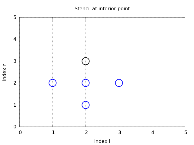
For uniformly distributed mesh points we can introduce the constant mesh spacings \(\Delta t\) and \(\Delta x\). We have that \[ x_i = i\Delta x,\ i=0,\ldots,N_x,\quad t_n = n\Delta t,\ n=0,\ldots,N_t\tp \] We also have that \(\Delta x = x_i-x_{i-1}\), \(i=1,\ldots,N_x\), and \(\Delta t = t_n - t_{n-1}\), \(n=1,\ldots,N_t\). Figure Figure 2.1 displays a mesh in the \(x,t\) plane with \(N_t=5\), \(N_x=5\), and constant mesh spacings.

2.3 The discrete solution

The solution \(u(x,t)\) is sought at the mesh points. We introduce the mesh function \(u_i^n\), which approximates the exact solution at the mesh point \((x_i,t_n)\) for \(i=0,\ldots,N_x\) and \(n=0,\ldots,N_t\). Using the finite difference method, we shall develop algebraic equations for computing the mesh function.

2.4 Fulfilling the equation at the mesh points

In the finite difference method, we relax the condition that (2.1) holds at all points in the space-time domain \((0,L)\times (0,T]\) to the requirement that the PDE is fulfilled at the interior mesh points only: \[ \frac{\partial^2}{\partial t^2} u(x_i, t_n) = c^2\frac{\partial^2}{\partial x^2} u(x_i, t_n), \tag{2.6}\] for \(i=1,\ldots,N_x-1\) and \(n=1,\ldots,N_t-1\). For \(n=0\) we have the initial conditions \(u=I(x)\) and \(u_t=0\), and at the boundaries \(i=0,N_x\) we have the boundary condition \(u=0\).

2.5 Replacing derivatives by finite differences

The second-order derivatives can be replaced by central differences. The most widely used difference approximation of the second-order derivative is \[ \frac{\partial^2}{\partial t^2}u(x_i,t_n)\approx \frac{u_i^{n+1} - 2u_i^n + u^{n-1}_i}{\Delta t^2}\tp \] It is convenient to introduce the finite difference operator notation \[ [D_tD_t u]^n_i = \frac{u_i^{n+1} - 2u_i^n + u^{n-1}_i}{\Delta t^2}\tp \] A similar approximation of the second-order derivative in the \(x\) direction reads \[ \frac{\partial^2}{\partial x^2}u(x_i,t_n)\approx \frac{u_{i+1}^{n} - 2u_i^n + u^{n}_{i-1}}{\Delta x^2} = [D_xD_x u]^n_i \tp \] ### Algebraic version of the PDE We can now replace the derivatives in (2.6) and get \[ \frac{u_i^{n+1} - 2u_i^n + u^{n-1}_i}{\Delta t^2} = c^2\frac{u_{i+1}^{n} - 2u_i^n + u^{n}_{i-1}}{\Delta x^2}, \tag{2.7}\] or written more compactly using the operator notation: \[ [D_tD_t u = c^2 D_xD_x]^{n}_i \tp \tag{2.8}\]

2.5.1 Interpretation of the equation as a stencil

A characteristic feature of (2.7) is that it involves \(u\) values from neighboring points only: \(u_i^{n+1}\), \(u^n_{i\pm 1}\), \(u^n_i\), and \(u^{n-1}_i\). The circles in Figure Figure 2.1 illustrate such neighboring mesh points that contribute to an algebraic equation. In this particular case, we have sampled the PDE at the point \((2,2)\) and constructed (2.7), which then involves a coupling of \(u_1^2\), \(u_2^3\), \(u_2^2\), \(u_2^1\), and \(u_3^2\). The term stencil is often used about the algebraic equation at a mesh point, and the geometry of a typical stencil is illustrated in Figure Figure 2.1. One also often refers to the algebraic equations as discrete equations, (finite) difference equations or a finite difference scheme.

Figure 2.1: Mesh in space and time. Filled circles represent known values from previous time steps; the empty circle is the unknown to be computed.

2.5.2 Algebraic version of the initial conditions

We also need to replace the derivative in the initial condition (2.3) by a finite difference approximation. A centered difference of the type \[ \frac{\partial}{\partial t} u(x_i,t_0)\approx \frac{u^1_i - u^{-1}_i}{2\Delta t} = [D_{2t} u]^0_i, \] seems appropriate. Writing out this equation and ordering the terms give \[ u^{-1}_i=u^{1}_i,\quad i=0,\ldots,N_x\tp \tag{2.9}\] The other initial condition can be computed by \[ u_i^0 = I(x_i),\quad i=0,\ldots,N_x\tp \]

2.6 Formulating a recursive algorithm

We assume that \(u^n_i\) and \(u^{n-1}_i\) are available for \(i=0,\ldots,N_x\). The only unknown quantity in (2.7) is therefore \(u^{n+1}_i\), which we now can solve for: \[ u^{n+1}_i = -u^{n-1}_i + 2u^n_i + C^2 \left(u^{n}_{i+1}-2u^{n}_{i} + u^{n}_{i-1}\right)\tp \tag{2.10}\] We have here introduced the parameter \[ C = c\frac{\Delta t}{\Delta x}, \] known as the Courant number.

\(C\) is the key parameter in the discrete wave equation

We see that the discrete version of the PDE features only one parameter, \(C\), which is therefore the key parameter, together with \(N_x\), that governs the quality of the numerical solution (see Section Section 2.40 for details). Both the primary physical parameter \(c\) and the numerical parameters \(\Delta x\) and \(\Delta t\) are lumped together in \(C\). Note that \(C\) is a dimensionless parameter.

Given that \(u^{n-1}_i\) and \(u^n_i\) are known for \(i=0,\ldots,N_x\), we find new values at the next time level by applying the formula (2.10) for \(i=1,\ldots,N_x-1\). Figure Figure 2.1 illustrates the points that are used to compute \(u^3_2\). For the boundary points, \(i=0\) and \(i=N_x\), we apply the boundary conditions \(u_i^{n+1}=0\).

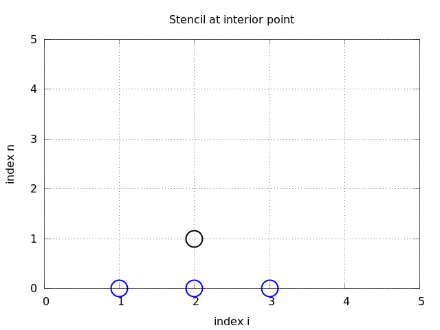
Even though sound reasoning leads up to (2.10), there is still a minor challenge with it that needs to be resolved. Think of the very first computational step to be made. The scheme (2.10) is supposed to start at \(n=1\), which means that we compute \(u^2\) from \(u^1\) and \(u^0\). Unfortunately, we do not know the value of \(u^1\), so how to proceed? A standard procedure in such cases is to apply (2.10) also for \(n=0\). This immediately seems strange, since it involves \(u^{-1}_i\), which is an undefined quantity outside the time mesh (and the time domain). However, we can use the initial condition (2.9) in combination with (2.10) when \(n=0\) to eliminate \(u^{-1}_i\) and arrive at a special formula for \(u_i^1\): \[ u_i^1 = u^0_i - \half C^2\left(u^{0}_{i+1}-2u^{0}_{i} + u^{0}_{i-1}\right) \tp \tag{2.11}\] Figure Figure 2.2 illustrates how (2.11) connects four instead of five points: \(u^1_2\), \(u_1^0\), \(u_2^0\), and \(u_3^0\).

Figure 2.2: Modified stencil for the first time step. Only values at \(n=0\) (initial condition) are needed since there is no \(n-1\) level yet.

We can now summarize the computational algorithm:

1. Compute \(u^0_i=I(x_i)\) for \(i=0,\ldots,N_x\)
2. Compute \(u^1_i\) by (2.11) for \(i=1,2,\ldots,N_x-1\) and set \(u_i^1=0\) for the boundary points given by \(i=0\) and \(i=N_x\),
3. For each time level \(n=1,2,\ldots,N_t-1\)
4. apply (2.10) to find \(u^{n+1}_i\) for \(i=1,\ldots,N_x-1\)
5. set \(u^{n+1}_i=0\) for the boundary points having \(i=0\), \(i=N_x\).

The algorithm essentially consists of moving a finite difference stencil through all the mesh points.

2.7 Sketch of an implementation

The algorithm only involves the three most recent time levels, so we need only three arrays for \(u_i^{n+1}\), \(u_i^n\), and \(u_i^{n-1}\), \(i=0,\ldots,N_x\). Storing all the solutions in a two-dimensional array of size \((N_x+1)\times (N_t+1)\) would be possible in this simple one-dimensional PDE problem, but is normally out of the question in three-dimensional (3D) and large two-dimensional (2D) problems. We shall therefore, in all our PDE solving programs, have the unknown in memory at as few time levels as possible.

In a Python implementation of this algorithm, we use the array elements u[i] to store \(u^{n+1}_i\), u_n[i] to store \(u^n_i\), and u_nm1[i] to store \(u^{n-1}_i\).

The following Python snippet realizes the steps in the computational algorithm.

dx = x[1] - x[0]
dt = t[1] - t[0]
C = c*dt/dx            # Courant number
Nt = len(t)-1
C2 = C**2              # Help variable in the scheme

for i in range(0, Nx+1):
    u_n[i] = I(x[i])

for i in range(1, Nx):
    u[i] = u_n[i] - \
           0.5*C**2 * (u_n[i+1] - 2*u_n[i] + u_n[i-1])
u[0] = 0;  u[Nx] = 0   # Enforce boundary conditions

u_nm1[:], u_n[:] = u_n, u

for n in range(1, Nt):
    for i in range(1, Nx):
        u[i] = 2*u_n[i] - u_nm1[i] - \
               C**2 * (u_n[i+1] - 2*u_n[i] + u_n[i-1])

    u[0] = 0;  u[Nx] = 0

    u_nm1[:], u_n[:] = u_n, u

Before implementing the algorithm, it is convenient to add a source term to the PDE (2.1), since that gives us more freedom in finding test problems for verification. Physically, a source term acts as a generator for waves in the interior of the domain.

2.8 A slightly generalized model problem

We now address the following extended initial-boundary value problem for one-dimensional wave phenomena:

\[ u_{tt} = c^2 u_{xx} + f(x,t), \quad x\in (0,L),\ t\in (0,T] \tag{2.12}\] \[ u(x,0) = I(x), \quad x\in [0,L] \tag{2.13}\] \[ u_t(x,0) = V(x), \quad x\in [0,L] \tag{2.14}\] \[ u(0,t) = 0, \quad t>0 \tag{2.15}\] \[ u(L,t) = 0, \quad t>0 \tag{2.16}\]

Sampling the PDE at \((x_i,t_n)\) and using the same finite difference approximations as above, yields \[ [D_tD_t u = c^2 D_xD_x u + f]^{n}_i \tp \tag{2.17}\] Writing this out and solving for the unknown \(u^{n+1}_i\) results in \[ u^{n+1}_i = -u^{n-1}_i + 2u^n_i + C^2 (u^{n}_{i+1}-2u^{n}_{i} + u^{n}_{i-1}) + \Delta t^2 f^n_i \tp \tag{2.18}\]

The equation for the first time step must be rederived. The discretization of the initial condition \(u_t = V(x)\) at \(t=0\) becomes \[ [D_{2t}u = V]^0_i\quad\Rightarrow\quad u^{-1}_i = u^{1}_i - 2\Delta t V_i, \] which, when inserted in (2.18) for \(n=0\), gives the special formula \[ u^{1}_i = u^0_i - \Delta t V_i + {\half} C^2 \left(u^{0}_{i+1}-2u^{0}_{i} + u^{0}_{i-1}\right) + \half\Delta t^2 f^0_i \tp \tag{2.19}\]

2.9 Using an analytical solution of physical significance

Many wave problems feature sinusoidal oscillations in time and space. For example, the original PDE problem (2.1)-(2.5) allows an exact solution \[ u_{\text{e}}(x,t) = A\sin\left(\frac{\pi}{L}x\right) \cos\left(\frac{\pi}{L}ct\right)\tp \tag{2.20}\] This \(u_{\text{e}}\) fulfills the PDE with \(f=0\), boundary conditions \(u_{\text{e}}(0,t)=u_{\text{e}}(L,t)=0\), as well as initial conditions \(I(x)=A\sin\left(\frac{\pi}{L}x\right)\) and \(V=0\).

How to use exact solutions for verification

It is common to use such exact solutions of physical interest to verify implementations. However, the numerical solution \(u^n_i\) will only be an approximation to \(u_{\text{e}}(x_i,t_n)\). We have no knowledge of the precise size of the error in this approximation, and therefore we can never know if discrepancies between \(u^n_i\) and \(u_{\text{e}}(x_i,t_n)\) are caused by mathematical approximations or programming errors. In particular, if plots of the computed solution \(u^n_i\) and the exact one (2.20) look similar, many are tempted to claim that the implementation works. However, even if color plots look nice and the accuracy is “deemed good”, there can still be serious programming errors present!

The only way to use exact physical solutions like (2.20) for serious and thorough verification is to run a series of simulations on finer and finer meshes, measure the integrated error in each mesh, and from this information estimate the empirical convergence rate of the method.

An introduction to the computing of convergence rates is given in Section 3.1.6 in (Langtangen 2016). There is also a detailed example on computing convergence rates in Section 1.5.

In the present problem, one expects the method to have a convergence rate of 2 (see Section Section 2.40), so if the computed rates are close to 2 on a sufficiently fine mesh, we have good evidence that the implementation is free of programming mistakes.

2.10 Manufactured solution and estimation of convergence rates

2.10.1 Specifying the solution and computing corresponding data

One problem with the exact solution (2.20) is that it requires a simplification (\(V=0, f=0\)) of the implemented problem (2.12)-(2.16). An advantage of using a manufactured solution is that we can test all terms in the PDE problem. The idea of this approach is to set up some chosen solution and fit the source term, boundary conditions, and initial conditions to be compatible with the chosen solution. Given that our boundary conditions in the implementation are \(u(0,t)=u(L,t)=0\), we must choose a solution that fulfills these conditions. One example is \[ u_{\text{e}}(x,t) = x(L-x)\sin t\tp \] Inserted in the PDE \(u_{tt}=c^2u_{xx}+f\) we get \[ -x(L-x)\sin t = -c^2 2\sin t + f\quad\Rightarrow f = (2c^2 - x(L-x))\sin t\tp \] The initial conditions become

\[\begin{align*} u(x,0) =& I(x) = 0,\\ u_t(x,0) &= V(x) = x(L-x)\tp \end{align*}\]

2.10.2 Defining a single discretization parameter

To verify the code, we compute the convergence rates in a series of simulations, letting each simulation use a finer mesh than the previous one. Such empirical estimation of convergence rates relies on an assumption that some measure \(E\) of the numerical error is related to the discretization parameters through \[ E = C_t\Delta t^r + C_x\Delta x^p, \] where \(C_t\), \(C_x\), \(r\), and \(p\) are constants. The constants \(r\) and \(p\) are known as the convergence rates in time and space, respectively. From the accuracy in the finite difference approximations, we expect \(r=p=2\), since the error terms are of order \(\Delta t^2\) and \(\Delta x^2\). This is confirmed by truncation error analysis and other types of analysis.

By using an exact solution of the PDE problem, we will next compute the error measure \(E\) on a sequence of refined meshes and see if the rates \(r=p=2\) are obtained. We will not be concerned with estimating the constants \(C_t\) and \(C_x\), simply because we are not interested in their values.

It is advantageous to introduce a single discretization parameter \(h=\Delta t=\hat c \Delta x\) for some constant \(\hat c\). Since \(\Delta t\) and \(\Delta x\) are related through the Courant number, \(\Delta t = C\Delta x/c\), we set \(h=\Delta t\), and then \(\Delta x = hc/C\). Now the expression for the error measure is greatly simplified: \[ E = C_t\Delta t^r + C_x\Delta x^r = C_t h^r + C_x\left(\frac{c}{C}\right)^r h^r = Dh^r,\quad D = C_t+C_x\left(\frac{c}{C}\right)^r \tp \] ### Computing errors We choose an initial discretization parameter \(h_0\) and run experiments with decreasing \(h\): \(h_i=2^{-i}h_0\), \(i=1,2,\ldots,m\). Halving \(h\) in each experiment is not necessary, but it is a common choice. For each experiment we must record \(E\) and \(h\). Standard choices of error measure are the \(\ell^2\) and \(\ell^\infty\) norms of the error mesh function \(e^n_i\):

\[ E = ||e^n_i||_{\ell^2} = \left( \Delta t\Delta x \sum_{n=0}^{N_t}\sum_{i=0}^{N_x} (e^n_i)^2\right)^{\half},\quad e^n_i = u_{\text{e}}(x_i,t_n)-u^n_i, \tag{2.21}\] \[ E = ||e^n_i||_{\ell^\infty} = \max_{i,n} |e^n_i|\tp \tag{2.22}\] In Python, one can compute \(\sum_{i}(e^{n}_i)^2\) at each time step and accumulate the value in some sum variable, say e2_sum. At the final time step one can do sqrt(dt*dx*e2_sum). For the \(\ell^\infty\) norm one must compare the maximum error at a time level (e.max()) with the global maximum over the time domain: e_max = max(e_max, e.max()).

An alternative error measure is to use a spatial norm at one time step only, e.g., the end time \(T\) (\(n=N_t\)):

\[\begin{align} E &= ||e^n_i||_{\ell^2} = \left( \Delta x\sum_{i=0}^{N_x} (e^n_i)^2\right)^{\half},\quad e^n_i = u_{\text{e}}(x_i,t_n)-u^n_i, \\ E &= ||e^n_i||_{\ell^\infty} = \max_{0\leq i\leq N_x} |e^{n}_i|\tp \end{align}\] The important point is that the error measure (\(E\)) for the simulation is represented by a single number.

2.10.3 Computing rates

Let \(E_i\) be the error measure in experiment (mesh) number \(i\) (not to be confused with the spatial index \(i\)) and let \(h_i\) be the corresponding discretization parameter (\(h\)). With the error model \(E_i = Dh_i^r\), we can estimate \(r\) by comparing two consecutive experiments:

\[\begin{align*} E_{i+1}& =D h_{i+1}^{r},\\ E_{i}& =D h_{i}^{r}\tp \end{align*}\] Dividing the two equations eliminates the (uninteresting) constant \(D\). Thereafter, solving for \(r\) yields \[ r = \frac{\ln E_{i+1}/E_{i}}{\ln h_{i+1}/h_{i}}\tp \] Since \(r\) depends on \(i\), i.e., which simulations we compare, we add an index to \(r\): \(r_i\), where \(i=0,\ldots,m-2\), if we have \(m\) experiments: \((h_0,E_0),\ldots,(h_{m-1}, E_{m-1})\).

In our present discretization of the wave equation we expect \(r=2\), and hence the \(r_i\) values should converge to 2 as \(i\) increases.

2.11 Constructing an exact solution of the discrete equations

With a manufactured or known analytical solution, as outlined above, we can estimate convergence rates and see if they have the correct asymptotic behavior. Experience shows that this is a quite good verification technique in that many common bugs will destroy the convergence rates. A significantly better test though, would be to check that the numerical solution is exactly what it should be. This will in general require exact knowledge of the numerical error, which we do not normally have (although we in Section Section 2.40 establish such knowledge in simple cases). However, it is possible to look for solutions where we can show that the numerical error vanishes, i.e., the solution of the original continuous PDE problem is also a solution of the discrete equations. This property often arises if the exact solution of the PDE is a lower-order polynomial. (Truncation error analysis leads to error measures that involve derivatives of the exact solution. In the present problem, the truncation error involves 4th-order derivatives of \(u\) in space and time. Choosing \(u\) as a polynomial of degree three or less will therefore lead to vanishing error.)

We shall now illustrate the construction of an exact solution to both the PDE itself and the discrete equations. Our chosen manufactured solution is quadratic in space and linear in time. More specifically, we set \[ u_{\text{e}} (x,t) = x(L-x)(1+{\half}t), \tag{2.23}\] which by insertion in the PDE leads to \(f(x,t)=2(1+t)c^2\). This \(u_{\text{e}}\) fulfills the boundary conditions \(u=0\) and demands \(I(x)=x(L-x)\) and \(V(x)={\half}x(L-x)\).

To realize that the chosen \(u_{\text{e}}\) is also an exact solution of the discrete equations, we first remind ourselves that \(t_n=n\Delta t\) so that

\[\begin{align} \lbrack D_tD_t t^2\rbrack^n &= \frac{t_{n+1}^2 - 2t_n^2 + t_{n-1}^2}{\Delta t^2} = (n+1)^2 -2n^2 + (n-1)^2 = 2,\\ \lbrack D_tD_t t\rbrack^n &= \frac{t_{n+1} - 2t_n + t_{n-1}}{\Delta t^2} = \frac{((n+1) -2n + (n-1))\Delta t}{\Delta t^2} = 0 \end{align}\] Hence, \[ [D_tD_t u_{\text{e}}]^n_i = x_i(L-x_i)[D_tD_t (1+{\half}t)]^n = x_i(L-x_i){\half}[D_tD_t t]^n = 0\tp \] Similarly, we get that

\[\begin{align*} \lbrack D_xD_x u_{\text{e}}\rbrack^n_i &= (1+{\half}t_n)\lbrack D_xD_x (xL-x^2)\rbrack_i\\ & = (1+{\half}t_n)\lbrack LD_xD_x x - D_xD_x x^2\rbrack_i \\ &= -2(1+{\half}t_n) \end{align*}\] Now, \(f^n_i = 2(1+{\half}t_n)c^2\), which results in \[ [D_tD_t u_{\text{e}} - c^2D_xD_xu_{\text{e}} - f]^n_i = 0 + c^2 2(1 + {\half}t_{n}) + 2(1+{\half}t_n)c^2 = 0\tp \] Moreover, \(u_{\text{e}}(x_i,0)=I(x_i)\), \(\partial u_{\text{e}}/\partial t = V(x_i)\) at \(t=0\), and \(u_{\text{e}}(x_0,t)=u_{\text{e}}(x_{N_x},0)=0\). Also the modified scheme for the first time step is fulfilled by \(u_{\text{e}}(x_i,t_n)\).

Therefore, the exact solution \(u_{\text{e}}(x,t)=x(L-x)(1+t/2)\) of the PDE problem is also an exact solution of the discrete problem. This means that we know beforehand what numbers the numerical algorithm should produce. We can use this fact to check that the computed \(u^n_i\) values from an implementation equals \(u_{\text{e}}(x_i,t_n)\), within machine precision. This result is valid regardless of the mesh spacings \(\Delta x\) and \(\Delta t\)! Nevertheless, there might be stability restrictions on \(\Delta x\) and \(\Delta t\), so the test can only be run for a mesh that is compatible with the stability criterion (which in the present case is \(C\leq 1\), to be derived later).

A product of quadratic or linear expressions in the various

independent variables, as shown above, will often fulfill both the PDE problem and the discrete equations, and can therefore be very useful solutions for verifying implementations.

However, for 1D wave equations of the type \(u_{tt}=c^2u_{xx}\) we shall see that there is always another much more powerful way of generating exact solutions (which consists in just setting \(C=1\) (!), as shown in Section Section 2.40).

2.12 Solving the Wave Equation with Devito

In this section we demonstrate how to solve the wave equation using the Devito domain-specific language (DSL). Devito allows us to write the PDE symbolically and generates optimized C code automatically.

2.12.1 From Mathematics to Devito Code

Recall the 1D wave equation from Section 2.1: \[ \frac{\partial^2 u}{\partial t^2} = c^2 \frac{\partial^2 u}{\partial x^2}, \quad x \in (0, L),\ t \in (0, T] \tag{2.24}\] with initial conditions \(u(x, 0) = I(x)\) and \(\partial u/\partial t|_{t=0} = V(x)\), and boundary conditions \(u(0, t) = u(L, t) = 0\).

In Devito, we express this PDE directly using symbolic derivatives. The key abstractions are:

• Grid: Defines the discrete domain
• TimeFunction: A field that varies in both space and time
• Eq: An equation relating symbolic expressions
• Operator: Compiles equations to optimized C code

2.12.2 The Devito Grid

A Devito Grid defines the discrete spatial domain:

from devito import Grid

L = 1.0      # Domain length
Nx = 100     # Number of grid intervals

grid = Grid(shape=(Nx + 1,), extent=(L,))

The shape is the number of grid points (including boundaries), and extent is the physical size of the domain.

2.12.3 TimeFunction for the Wave Field

The solution \(u(x, t)\) is represented by a TimeFunction:

from devito import TimeFunction

u = TimeFunction(name='u', grid=grid, time_order=2, space_order=2)

The key parameters are:

• time_order=2: We need \(u^{n+1}\), \(u^n\), \(u^{n-1}\) for the wave equation
• space_order=2: Central difference with second-order accuracy

2.12.4 Symbolic Derivatives

Devito provides symbolic access to derivatives through attribute notation:

Derivative	Devito syntax	Mathematical meaning
First time	u.dt	\(\partial u/\partial t\)
Second time	u.dt2	\(\partial^2 u/\partial t^2\)
First space	u.dx	\(\partial u/\partial x\)
Second space	u.dx2	\(\partial^2 u/\partial x^2\)

2.12.5 Formulating the PDE

We express the wave equation as a residual that should be zero:

from devito import Eq, solve, Constant

c_sq = Constant(name='c_sq')  # Wave speed squared

# PDE: u_tt - c^2 * u_xx = 0
pde = u.dt2 - c_sq * u.dx2

The solve function isolates the unknown \(u^{n+1}\):

stencil = Eq(u.forward, solve(pde, u.forward))

Here u.forward represents \(u^{n+1}\), the solution at the next time level.

2.12.6 Boundary Conditions

For Dirichlet conditions \(u(0, t) = u(L, t) = 0\), we add explicit equations:

t_dim = grid.stepping_dim  # Time index dimension

bc_left = Eq(u[t_dim + 1, 0], 0)
bc_right = Eq(u[t_dim + 1, Nx], 0)

2.12.7 Creating and Running the Operator

The Operator compiles all equations into optimized code:

from devito import Operator

op = Operator([stencil, bc_left, bc_right])

To execute a time step, we call:

op.apply(time_m=1, time_M=1, dt=dt, c_sq=c**2)

2.12.8 Complete Solver Implementation

The module src.wave provides a complete solver that handles:

• Initial conditions with velocity (\(u_t(x, 0) = V(x)\))
• CFL stability checking
• Optional history storage

from src.wave import solve_wave_1d
import numpy as np

# Define initial condition: plucked string
def I(x):
    return np.sin(np.pi * x)

# Solve
result = solve_wave_1d(
    L=1.0,           # Domain length
    c=1.0,           # Wave speed
    Nx=100,          # Grid points
    T=1.0,           # Final time
    C=0.9,           # Courant number
    I=I,             # Initial displacement
)

# Access results
u_final = result.u   # Solution at final time
x = result.x         # Spatial grid

2.12.9 The Courant Number and Stability

The Courant number \(C = c \Delta t / \Delta x\) determines stability. For the explicit wave equation solver, we require \(C \le 1\).

When \(C = 1\) (the magic value), the numerical solution is exact for waves traveling in either direction. This is because the domain of dependence of the numerical scheme exactly matches the physical domain of dependence.

2.12.10 Handling Initial Velocity

The first time step requires special treatment when \(V(x) \ne 0\). Using the Taylor expansion: \[ u^1 = u^0 + \Delta t \cdot V(x) + \frac{1}{2} \Delta t^2 c^2 u_{xx}^0 \]

The solver implements this as:

u0 = I(x_coords)
v0 = V(x_coords)
u_xx_0 = np.zeros_like(u0)
u_xx_0[1:-1] = (u0[2:] - 2*u0[1:-1] + u0[:-2]) / dx**2

u1 = u0 + dt * v0 + 0.5 * dt**2 * c**2 * u_xx_0

2.12.11 Verification: Standing Wave Solution

The standing wave with \(I(x) = A \sin(\pi x / L)\) and \(V = 0\) has the exact solution: \[ u(x, t) = A \sin\left(\frac{\pi x}{L}\right) \cos\left(\frac{\pi c t}{L}\right) \]

We can verify our implementation converges at the expected rate:

from src.wave import convergence_test_wave_1d

grid_sizes, errors, rate = convergence_test_wave_1d(
    grid_sizes=[20, 40, 80, 160],
    T=0.5,
    C=0.9,
)

print(f"Observed convergence rate: {rate:.2f}")  # Should be ~2.0

2.12.12 Visualization

For time-dependent problems, animation is essential. With the history saved, we can create animations:

import matplotlib.pyplot as plt
from matplotlib.animation import FuncAnimation

result = solve_wave_1d(
    L=1.0, c=1.0, Nx=100, T=2.0, C=0.9,
    save_history=True,
)

fig, ax = plt.subplots()
line, = ax.plot(result.x, result.u_history[0])
ax.set_ylim(-1.2, 1.2)
ax.set_xlabel('x')
ax.set_ylabel('u')

def update(frame):
    line.set_ydata(result.u_history[frame])
    ax.set_title(f't = {result.t_history[frame]:.3f}')
    return line,

anim = FuncAnimation(fig, update, frames=len(result.t_history),
                     interval=50, blit=True)

2.12.13 Summary: Devito vs. NumPy

The key advantages of using Devito for wave equations:

1. Symbolic PDEs: Write the math, not the stencils
2. Automatic optimization: Cache-efficient loops generated automatically
3. Parallelization: OpenMP/MPI/GPU support without code changes
4. Dimension-agnostic: Same code pattern works for 1D, 2D, 3D

The explicit time-stepping loop remains visible to the user for educational purposes, but Devito handles the spatial discretization and can generate highly optimized code for the inner loop.

2.12.14 Neumann Boundary Conditions

For Neumann boundary conditions \(\partial u/\partial x = 0\) at the boundaries, Devito can use ghost points or modified stencils. The ghost point approach extends the grid with extra points outside the domain:

from devito import Grid, TimeFunction, Eq, solve, Operator

# Grid with ghost points for Neumann BCs
Nx = 100
grid = Grid(shape=(Nx + 3,), extent=(1.0,))  # Extra points at each end
u = TimeFunction(name='u', grid=grid, time_order=2, space_order=2)

# PDE for interior points
pde = u.dt2 - c**2 * u.dx2
stencil = Eq(u.forward, solve(pde, u.forward))

# Neumann BCs: u[0] = u[2] and u[-1] = u[-3]
bc_left = Eq(u.forward[0], u.forward[2])
bc_right = Eq(u.forward[Nx+2], u.forward[Nx])

op = Operator([stencil, bc_left, bc_right])

The symmetry condition \(u_{-1} = u_1\) effectively implements the zero-derivative condition at the boundary.

2.12.15 Verification with Exact Solutions

The most rigorous verification approach uses solutions that the numerical method should reproduce exactly. For the wave equation, a quadratic polynomial in space and linear in time works:

\[ u_{\text{exact}}(x, t) = x(L-x)(1 + t/2) \]

This satisfies: - Boundary conditions: \(u(0,t) = u(L,t) = 0\) - Initial condition: \(I(x) = x(L-x)\) - Initial velocity: \(V(x) = \frac{1}{2}x(L-x)\)

The source term \(f(x,t)\) is found by substitution into the PDE: \[ f(x,t) = 2c^2(1 + t/2) \]

Since the finite difference truncation error involves fourth-order derivatives (which vanish for polynomials of degree 3 or less), the numerical solution should match the exact solution to machine precision:

import numpy as np

def test_quadratic_solution():
    """Verify solver with exact polynomial solution."""
    L, c = 2.5, 1.5
    C = 0.75
    Nx = 20
    T = 2.0

    def u_exact(x, t):
        return x * (L - x) * (1 + 0.5 * t)

    def I(x):
        return u_exact(x, 0)

    def V(x):
        return 0.5 * x * (L - x)

    def f(x, t):
        return 2 * c**2 * (1 + 0.5 * t)

    result = solve_wave_1d(L=L, c=c, Nx=Nx, T=T, C=C, I=I, V=V, f=f)

    error = np.abs(result.u - u_exact(result.x, T)).max()
    assert error < 1e-12, f"Error {error} exceeds tolerance"

2.12.16 Convergence Rate Testing

For more general solutions, we verify the expected \(O(\Delta x^2 + \Delta t^2)\) convergence rate by running simulations on successively refined meshes:

def compute_convergence_rate(errors, h_values):
    """Compute convergence rate from error sequence."""
    rates = []
    for i in range(1, len(errors)):
        rate = np.log(errors[i-1] / errors[i]) / np.log(h_values[i-1] / h_values[i])
        rates.append(rate)
    return rates

# Run with mesh refinement
grid_sizes = [20, 40, 80, 160, 320]
errors = []

for Nx in grid_sizes:
    result = solve_wave_1d(L=1.0, c=1.0, Nx=Nx, T=0.5, C=0.9, I=I)
    error = np.abs(result.u - u_exact(result.x, 0.5)).max()
    errors.append(error)

rates = compute_convergence_rate(errors, [1.0/Nx for Nx in grid_sizes])
print(f"Observed rates: {rates}")  # Should approach 2.0

Automatic Optimization

Devito generates optimized C code with cache-efficient loops and parallelization. This replaces manual NumPy vectorization while achieving better performance on modern hardware.

2.13 Source Terms and Variable Coefficients

Real-world wave propagation often involves source terms and spatially varying wave speeds. This section extends the Devito wave solver to handle these features.

2.13.1 Adding a Source Term

The wave equation with a source term is: \[ \frac{\partial^2 u}{\partial t^2} = c^2 \frac{\partial^2 u}{\partial x^2} + f(x, t) \tag{2.25}\]

In seismic applications, \(f(x, t)\) often represents an impulsive source at a specific location.

2.13.2 Source Wavelets

The src.wave module provides common source wavelets used in seismic modeling:

from src.wave import ricker_wavelet, gaussian_pulse
import numpy as np

t = np.linspace(0, 0.5, 501)  # Time array

# Ricker wavelet with 25 Hz peak frequency
src_ricker = ricker_wavelet(t, f0=25.0)

# Gaussian pulse
src_gauss = gaussian_pulse(t, t0=0.1, sigma=0.02)

2.13.3 The Ricker Wavelet

The Ricker wavelet (Mexican hat wavelet) is the negative normalized second derivative of a Gaussian: \[ r(t) = A \left(1 - 2\pi^2 f_0^2 (t - t_0)^2\right) e^{-\pi^2 f_0^2 (t - t_0)^2} \]

where \(f_0\) is the peak frequency and \(t_0\) is the time shift.

import matplotlib.pyplot as plt
from src.wave import ricker_wavelet, get_source_spectrum

t = np.linspace(0, 0.3, 301)
dt = t[1] - t[0]

# Create wavelet
wavelet = ricker_wavelet(t, f0=25.0)

# Compute spectrum
freq, amp = get_source_spectrum(wavelet, dt)

fig, (ax1, ax2) = plt.subplots(1, 2, figsize=(10, 4))
ax1.plot(t, wavelet)
ax1.set_xlabel('Time (s)')
ax1.set_ylabel('Amplitude')
ax1.set_title('Ricker Wavelet (f0 = 25 Hz)')

ax2.plot(freq[:100], amp[:100])
ax2.set_xlabel('Frequency (Hz)')
ax2.set_ylabel('Amplitude')
ax2.set_title('Frequency Spectrum')
ax2.axvline(25, color='r', linestyle='--', label='Peak freq')
ax2.legend()

2.13.4 Point Sources in Devito

For seismic modeling, sources are often located at specific points in space. Devito provides SparseTimeFunction for this:

from devito import SparseTimeFunction

# Point source at x = 0.5
src = SparseTimeFunction(
    name='src', grid=grid,
    npoint=1, nt=Nt,
    coordinates=np.array([[0.5]])
)

# Set source wavelet
src.data[:] = ricker_wavelet(t, f0=25.0).reshape(-1, 1)

# Inject into the wave equation
src_term = src.inject(field=u.forward, expr=src * dt**2)

2.13.5 Variable Wave Speed

In heterogeneous media, the wave speed varies in space: \[ \frac{\partial^2 u}{\partial t^2} = \nabla \cdot (c^2(x) \nabla u) \]

In 1D, this simplifies to: \[ u_{tt} = (c^2 u_x)_x = c^2 u_{xx} + 2 c c_x u_x \]

For smoothly varying \(c(x)\), we can approximate this as: \[ u_{tt} \approx c^2(x) u_{xx} \]

2.13.6 Implementing Variable Velocity in Devito

We use a Function (not TimeFunction) for the velocity field:

from devito import Function

# Velocity field
c = Function(name='c', grid=grid)

# Set velocity values (e.g., layer model)
x_coords = np.linspace(0, L, Nx + 1)
c.data[:] = np.where(x_coords < 0.5, 1.0, 2.0)  # Two layers

The PDE uses this spatially varying velocity:

pde = u.dt2 - c**2 * u.dx2
stencil = Eq(u.forward, solve(pde, u.forward))

2.13.7 CFL Condition with Variable Velocity

When velocity varies, the CFL condition must use the maximum velocity: \[ \Delta t \le \frac{\Delta x}{c_{\max}} \]

c_max = np.max(c.data)
dt_stable = dx / c_max

2.13.8 Example: Wave Propagation in Layered Medium

Consider a domain with two layers of different wave speeds:

from devito import Grid, TimeFunction, Function, Eq, solve, Operator

# Setup
L = 2.0
Nx = 200
grid = Grid(shape=(Nx + 1,), extent=(L,))

# Velocity: slow layer (c=1) then fast layer (c=2)
c = Function(name='c', grid=grid)
x_coords = np.linspace(0, L, Nx + 1)
c.data[:] = np.where(x_coords < 1.0, 1.0, 2.0)

# Wave field
u = TimeFunction(name='u', grid=grid, time_order=2, space_order=2)

# Initial condition: Gaussian pulse in slow region
sigma = 0.1
x0 = 0.3
u.data[0, :] = np.exp(-((x_coords - x0) / sigma)**2)
u.data[1, :] = u.data[0, :]

# Wave equation with variable velocity
pde = u.dt2 - c**2 * u.dx2
stencil = Eq(u.forward, solve(pde, u.forward))

# Boundary conditions
bc_left = Eq(u[grid.stepping_dim + 1, 0], 0)
bc_right = Eq(u[grid.stepping_dim + 1, Nx], 0)

# Operator
op = Operator([stencil, bc_left, bc_right])

When the pulse reaches the interface at \(x = 1\):

1. Part of the wave is reflected back into the slow medium
2. Part of the wave is transmitted into the fast medium
3. The transmitted wave travels faster and has a different wavelength

2.13.9 Reflection and Transmission Coefficients

At an interface between media with velocities \(c_1\) and \(c_2\), the reflection coefficient is: \[ R = \frac{c_2 - c_1}{c_2 + c_1} \]

And the transmission coefficient is: \[ T = \frac{2 c_2}{c_2 + c_1} \]

For our example with \(c_1 = 1\) and \(c_2 = 2\):

• \(R = (2 - 1)/(2 + 1) = 1/3\)
• \(T = 2 \cdot 2/(2 + 1) = 4/3\)

The transmitted wave has larger amplitude but carries the same energy (accounting for the velocity change).

2.13.10 Absorbing Boundary Conditions

For open-domain problems, we want waves to leave without reflecting from artificial boundaries. A simple approach is a sponge layer (or damping layer) that gradually damps the solution near boundaries (Cerjan et al. 1985; Sochacki et al. 1987). For a comprehensive treatment of absorbing boundary conditions including damping layers, PML, and higher-order methods, see Section 2.50.

from devito import Function

# Damping coefficient (zero in interior, increasing at boundaries)
damp = Function(name='damp', grid=grid)

pad = 20  # Width of sponge layer
sigma_max = 3.0 * c / (pad * dx)  # Theory-based choice
damp_profile = np.zeros(Nx + 1)
for i in range(pad):
    d = (pad - i) / pad
    damp_profile[i] = sigma_max * d**3        # Left ramp
    damp_profile[Nx - i] = sigma_max * d**3   # Right ramp
damp.data[:] = damp_profile

# Modified PDE with damping term
pde_damped = u.dt2 + damp * u.dt - c**2 * u.dx2

The damping term \(\gamma u_t\) removes energy from the wave as it enters the sponge layer. The cubic polynomial ramp and the choice \(\sigma_{\max} = 3c/W\) ensure a smooth impedance transition; see Section 2.50.3 for a detailed treatment in 2D.

2.13.11 Summary

Devito makes it straightforward to extend the basic wave solver to handle:

• Source terms: Point sources and wavelets for seismic modeling
• Variable velocity: Layered or smooth velocity variations
• Absorbing boundaries: Sponge layers to reduce reflections

The key is that Devito handles the discretization automatically once we express the PDE symbolically. This allows us to focus on the physics rather than implementation details.

2.14 Neumann boundary conditions

Source Files

The verification and convergence testing functions presented in this chapter (test_plug, convergence_rates, PlotAndStoreSolution) demonstrate important software engineering practices. For Devito-based wave solvers with comprehensive tests, see src/wave/wave1D_devito.py and tests/test_wave_devito.py.

The boundary condition \(u=0\) in a wave equation reflects the wave, but \(u\) changes sign at the boundary, while the condition \(u_x=0\) reflects the wave as a mirror and preserves the sign.

Why is it so? Consider the boundary \(x=0\) and the condition \(u=0\). How will two values \(u(0, t)\) and \(u(\Delta x, t\) change from time \(t\) to \(t+\Delta t\)? Since \(u(0,t)=0\), \(u(\Delta x, t)\) and \(u(\Delta x, t+\Delta t)\) will be close to zero too. Their average in time must also be close to zero, especially in the limit \(\Delta x,\Delta t\rightarrow 0\): \[ \frac{1}{2}(u(\Delta x, t) + u(\Delta x, t+\Delta t))\approx 0\quad \Rightarrow\quad u(\Delta x, t+\Delta t) = -u(\Delta x, t)\tp \] This tells that \(u\) changes sign in time close to the boundary (otherwise the average would be larger than the \(u\) values and this is not compatible with keeping neighboring value \(u(0,t)\) fixed at zero).

For a Neumann condition \(u_x=0\) at \(x=0\) we consider the values \(u(0,t)\), \(u(\Delta x, t)\), \(u(0, t+\Delta t)\) and \(u(\Delta x,t+\Delta t)\). Now the boundary condition demands \(u(0,t) \approx u(\Delta x, t)\) and \(u(0, t+\Delta t) \approx u(\Delta x,t+\Delta t)\) to always get a flat spatial derivative.

Our next task is to explain how to implement the boundary condition \(u_x=0\), which is more complicated to express numerically and also to implement than a given value of \(u\). We shall present two methods for implementing \(u_x=0\) in a finite difference scheme, one based on deriving a modified stencil at the boundary, and another one based on extending the mesh with ghost cells and ghost points.

2.15 Neumann boundary condition

When a wave hits a boundary and is to be reflected back, one applies the condition \[ \frac{\partial u}{\partial n} \equiv \normalvec\cdot\nabla u = 0 \tp \tag{2.26}\] The derivative \(\partial /\partial n\) is in the outward normal direction from a general boundary. For a 1D domain \([0,L]\), we have that \[ \left.\frac{\partial}{\partial n}\right\vert_{x=L} = \left.\frac{\partial}{\partial x}\right\vert_{x=L},\quad \left.\frac{\partial}{\partial n}\right\vert_{x=0} = - \left.\frac{\partial}{\partial x}\right\vert_{x=0}\tp \]

Boundary condition terminology

Boundary conditions that specify the value of \(\partial u/\partial n\) (or shorter \(u_n\)) are known as Neumann conditions, while Dirichlet conditions refer to specifications of \(u\). When the values are zero (\(\partial u/\partial n=0\) or \(u=0\)) we speak about homogeneous Neumann or Dirichlet conditions.

2.16 Discretization of derivatives at the boundary

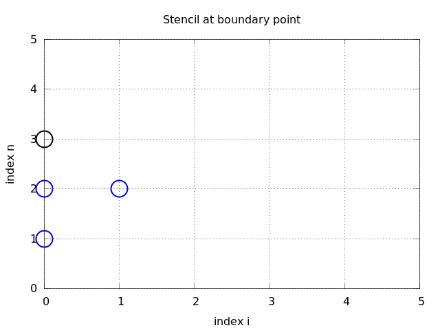
How can we incorporate the condition (2.26) in the finite difference scheme? Since we have used central differences in all the other approximations to derivatives in the scheme, it is tempting to implement (2.26) at \(x=0\) and \(t=t_n\) by the difference \[ [D_{2x} u]^n_0 = \frac{u_{-1}^n - u_1^n}{2\Delta x} = 0 \tp \tag{2.27}\] The problem is that \(u_{-1}^n\) is not a \(u\) value that is being computed since the point is outside the mesh. However, if we combine (2.27) with the scheme \[ u^{n+1}_i = -u^{n-1}_i + 2u^n_i + C^2 \left(u^{n}_{i+1}-2u^{n}_{i} + u^{n}_{i-1}\right), \tag{2.28}\] for \(i=0\), we can eliminate the fictitious value \(u_{-1}^n\). We see that \(u_{-1}^n=u_1^n\) from (2.27), which can be used in (2.28) to arrive at a modified scheme for the boundary point \(u_0^{n+1}\): \[ u^{n+1}_i = -u^{n-1}_i + 2u^n_i + 2C^2 \left(u^{n}_{i+1}-u^{n}_{i}\right),\quad i=0 \tp \] Figure Figure 2.3 visualizes this equation for computing \(u^3_0\) in terms of \(u^2_0\), \(u^1_0\), and \(u^2_1\).

Figure 2.3: Modified stencil at a boundary with a Neumann condition. The ghost point \(u_{-1}^n\) is eliminated using \(u_{-1}^n = u_1^n\).

Similarly, (2.26) applied at \(x=L\) is discretized by a central difference \[ \frac{u_{N_x+1}^n - u_{N_x-1}^n}{2\Delta x} = 0 \tp \tag{2.29}\] Combined with the scheme for \(i=N_x\) we get a modified scheme for the boundary value \(u_{N_x}^{n+1}\): \[ u^{n+1}_i = -u^{n-1}_i + 2u^n_i + 2C^2 \left(u^{n}_{i-1}-u^{n}_{i}\right),\quad i=N_x \tp \] The modification of the scheme at the boundary is also required for the special formula for the first time step.

2.17 Implementation of Neumann conditions

We have seen in the preceding section that the special formulas for the boundary points arise from replacing \(u_{i-1}^n\) by \(u_{i+1}^n\) when computing \(u_i^{n+1}\) from the stencil formula for \(i=0\). Similarly, we replace \(u_{i+1}^n\) by \(u_{i-1}^n\) in the stencil formula for \(i=N_x\). This observation can conveniently be used in the coding: we just work with the general stencil formula, but write the code such that it is easy to replace u[i-1] by u[i+1] and vice versa. This is achieved by having the indices i+1 and i-1 as variables ip1 (i plus 1) and im1 (i minus 1), respectively. At the boundary we can easily define im1=i+1 while we use im1=i-1 in the internal parts of the mesh. Here are the details of the implementation (note that the updating formula for u[i] is the general stencil formula):

i = 0
ip1 = i+1
im1 = ip1  # i-1 -> i+1
u[i] = u_n[i] + C2*(u_n[im1] - 2*u_n[i] + u_n[ip1])

i = Nx
im1 = i-1
ip1 = im1  # i+1 -> i-1
u[i] = u_n[i] + C2*(u_n[im1] - 2*u_n[i] + u_n[ip1])

We can in fact create one loop over both the internal and boundary points and use only one updating formula:

for i in range(0, Nx+1):
    ip1 = i+1 if i < Nx else i-1
    im1 = i-1 if i > 0  else i+1
    u[i] = u_n[i] + C2*(u_n[im1] - 2*u_n[i] + u_n[ip1])

For a complete implementation of Neumann boundary conditions using Devito, see Section 2.12 in the wave equation chapter. Devito handles boundary conditions through SubDomains, which provide a clean separation between interior updates and boundary treatment.

2.18 Index set notation

To improve our mathematical writing and our implementations, it is wise to introduce a special notation for index sets. This means that we write \(x_i\), followed by \(i\in\Ix\), instead of \(i=0,\ldots,N_x\). Obviously, \(\Ix\) must be the index set \(\Ix =\{0,\ldots,N_x\}\), but it is often advantageous to have a symbol for this set rather than specifying all its elements (all the time, as we have done up to now). This new notation saves writing and makes specifications of algorithms and their implementation as computer code simpler.

The first index in the set will be denoted \(\setb{\Ix}\) and the last \(\sete{\Ix}\). When we need to skip the first element of the set, we use \(\setr{\Ix}\) for the remaining subset \(\setr{\Ix}=\{1,\ldots,N_x\}\). Similarly, if the last element is to be dropped, we write \(\setl{\Ix}=\{0,\ldots,N_x-1\}\) for the remaining indices. All the indices corresponding to inner grid points are specified by \(\seti{\Ix}=\{1,\ldots,N_x-1\}\). For the time domain we find it natural to explicitly use 0 as the first index, so we will usually write \(n=0\) and \(t_0\) rather than \(n=\It^0\). We also avoid notation like \(x_{\sete{\Ix}}\) and will instead use \(x_i\), \(i=\sete{\Ix}\).

The Python code associated with index sets applies the following conventions:

Notation	Python
\(\Ix\)	Ix
\(\setb{\Ix}\)	Ix[0]
\(\sete{\Ix}\)	Ix[-1]
\(\setl{\Ix}\)	Ix[:-1]
\(\setr{\Ix}\)	Ix[1:]
\(\seti{\Ix}\)	Ix[1:-1]

Why index sets are useful

An important feature of the index set notation is that it keeps our formulas and code independent of how we count mesh points. For example, the notation \(i\in\Ix\) or \(i=\setb{\Ix}\) remains the same whether \(\Ix\) is defined as above or as starting at 1, i.e., \(\Ix=\{1,\ldots,Q\}\). Similarly, we can in the code define Ix=range(Nx+1) or Ix=range(1,Q), and expressions like Ix[0] and Ix[1:-1] remain correct. One application where the index set notation is convenient is conversion of code from a language where arrays has base index 0 (e.g., Python and C) to languages where the base index is 1 (e.g., MATLAB and Fortran). Another important application is implementation of Neumann conditions via ghost points (see next section).

For the current problem setting in the \(x,t\) plane, we work with the index sets \[ \Ix = \{0,\ldots,N_x\},\quad \It = \{0,\ldots,N_t\}, \] defined in Python as

Ix = range(0, Nx+1)
It = range(0, Nt+1)

A finite difference scheme can with the index set notation be specified as

\[\begin{align*} u_i^{n+1} &= u^n_i - \half C^2\left(u^{n}_{i+1}-2u^{n}_{i} + u^{n}_{i-1}\right),\quad, i\in\seti{\Ix},\ n=0,\\ u^{n+1}_i &= -u^{n-1}_i + 2u^n_i + C^2 \left(u^{n}_{i+1}-2u^{n}_{i}+u^{n}_{i-1}\right), \quad i\in\seti{\Ix},\ n\in\seti{\It},\\ u_i^{n+1} &= 0, \quad i=\setb{\Ix},\ n\in\setl{\It},\\ u_i^{n+1} &= 0, \quad i=\sete{\Ix},\ n\in\setl{\It}\tp \end{align*}\] The corresponding implementation becomes

for i in Ix[1:-1]:
    u[i] = u_n[i] - 0.5*C2*(u_n[i-1] - 2*u_n[i] + u_n[i+1])

for n in It[1:-1]:
    for i in Ix[1:-1]:
        u[i] = - u_nm1[i] + 2*u_n[i] + \
               C2*(u_n[i-1] - 2*u_n[i] + u_n[i+1])
    i = Ix[0];  u[i] = 0
    i = Ix[-1]; u[i] = 0

Boundary conditions in Devito

The 1D wave equation \(u_{tt}=c^2u_{xx}+f(x,t)\) with general boundary and initial conditions can be solved using Devito. See Section 2.12 for the implementation that handles:

• \(x=0\): \(u=U_0(t)\) or \(u_x=0\)
• \(x=L\): \(u=U_L(t)\) or \(u_x=0\)
• \(t=0\): \(u=I(x)\)
• \(t=0\): \(u_t=V(x)\)

Common test cases include:

• A rectangular plug-shaped initial condition. (For \(C=1\) the solution will be a rectangle that jumps one cell per time step, making the case well suited for verification.)
• A Gaussian function as initial condition.
• A triangular profile as initial condition, which resembles the typical initial shape of a guitar string.

2.19 Verifying the implementation of Neumann conditions

How can we test that the Neumann conditions are correctly implemented? It is tempting to apply a quadratic solution as described in Section 2.11, but it turns out that this solution is no longer an exact solution of the discrete equations if a Neumann condition is implemented on the boundary. A linear solution does not help since we only have homogeneous Neumann conditions, and we are consequently left with testing just a constant solution: \(u=\text{const}\).

The quadratic solution is very useful for testing, but it requires Dirichlet conditions at both ends.

Another test may utilize the fact that the approximation error vanishes when the Courant number is unity. We can, for example, start with a plug profile as initial condition, let this wave split into two plug waves, one in each direction, and check that the two plug waves come back and form the initial condition again after “one period” of the solution process. Neumann conditions can be applied at both ends. A proper test function reads

def test_plug():
    """Check that an initial plug is correct back after one period."""
    L = 1.0
    c = 0.5
    dt = (L / 10) / c  # Nx=10
    I = lambda x: 0 if abs(x - L / 2.0) > 0.1 else 1

    u_s, x, t, cpu = solver(
        I=I,
        V=None,
        f=None,
        c=0.5,
        U_0=None,
        U_L=None,
        L=L,
        dt=dt,
        C=1,
        T=4,
        user_action=None,
        version="scalar",
    )
    u_v, x, t, cpu = solver(
        I=I,
        V=None,
        f=None,
        c=0.5,
        U_0=None,
        U_L=None,
        L=L,
        dt=dt,
        C=1,
        T=4,
        user_action=None,
        version="vectorized",
    )
    tol = 1e-13
    diff = abs(u_s - u_v).max()
    assert diff < tol
    u_0 = np.array([I(x_) for x_ in x])
    diff = np.abs(u_s - u_0).max()
    assert diff < tol

Other tests must rely on an unknown approximation error, so effectively we are left with tests on the convergence rate.

2.20 Alternative implementation via ghost cells

2.20.1 Idea

Instead of modifying the scheme at the boundary, we can introduce extra points outside the domain such that the fictitious values \(u_{-1}^n\) and \(u_{N_x+1}^n\) are defined in the mesh. Adding the intervals \([-\Delta x,0]\) and \([L, L+\Delta x]\), known as ghost cells, to the mesh gives us all the needed mesh points, corresponding to \(i=-1,0,\ldots,N_x,N_x+1\). The extra points with \(i=-1\) and \(i=N_x+1\) are known as ghost points, and values at these points, \(u_{-1}^n\) and \(u_{N_x+1}^n\), are called ghost values.

The important idea is to ensure that we always have \[ u_{-1}^n = u_{1}^n\text{ and } u_{N_x+1}^n = u_{N_x-1}^n, \] because then the application of the standard scheme at a boundary point \(i=0\) or \(i=N_x\) will be correct and guarantee that the solution is compatible with the boundary condition \(u_x=0\).

Some readers may find it strange to just extend the domain with ghost cells as a general technique, because in some problems there is a completely different medium with different physics and equations right outside of a boundary. Nevertheless, one should view the ghost cell technique as a purely mathematical technique, which is valid in the limit \(\Delta x \rightarrow 0\) and helps us to implement derivatives.

2.20.2 Implementation

The u array now needs extra elements corresponding to the ghost points. Two new point values are needed:

u   = zeros(Nx+3)

The arrays u_n and u_nm1 must be defined accordingly.

Unfortunately, a major indexing problem arises with ghost cells. The reason is that Python indices must start at 0 and u[-1] will always mean the last element in u. This fact gives, apparently, a mismatch between the mathematical indices \(i=-1,0,\ldots,N_x+1\) and the Python indices running over u: 0,..,Nx+2. One remedy is to change the mathematical indexing of \(i\) in the scheme and write \[ u^{n+1}_i = \cdots,\quad i=1,\ldots,N_x+1, \] instead of \(i=0,\ldots,N_x\) as we have previously used. The ghost points now correspond to \(i=0\) and \(i=N_x+1\). A better solution is to use the ideas of Section Section 2.18: we hide the specific index value in an index set and operate with inner and boundary points using the index set notation.

To this end, we define u with proper length and Ix to be the corresponding indices for the real physical mesh points (\(1,2,\ldots,N_x+1\)):

u = zeros(Nx+3)
Ix = range(1, u.shape[0]-1)

That is, the boundary points have indices Ix[0] and Ix[-1] (as before). We first update the solution at all physical mesh points (i.e., interior points in the mesh):

for i in Ix:
    u[i] = - u_nm1[i] + 2*u_n[i] + \
           C2*(u_n[i-1] - 2*u_n[i] + u_n[i+1])

The indexing becomes a bit more complicated when we call functions like V(x) and f(x, t), as we must remember that the appropriate \(x\) coordinate is given as x[i-Ix[0]]:

for i in Ix:
    u[i] = u_n[i] + dt*V(x[i-Ix[0]]) + \
           0.5*C2*(u_n[i-1] - 2*u_n[i] + u_n[i+1]) + \
           0.5*dt2*f(x[i-Ix[0]], t[0])

It remains to update the solution at ghost points, i.e., u[0] and u[-1] (or u[Nx+2]). For a boundary condition \(u_x=0\), the ghost value must equal the value at the associated inner mesh point. Computer code makes this statement precise:

i = Ix[0]          # x=0 boundary
u[i-1] = u[i+1]
i = Ix[-1]         # x=L boundary
u[i+1] = u[i-1]

The physical solution to be plotted is now in u[1:-1], or equivalently u[Ix[0]:Ix[-1]+1], so this slice is the quantity to be returned from a solver function. In Devito, ghost cells are handled automatically through the halo region mechanism. See Section 2.12 for the Devito implementation.

We have to be careful with how the spatial and temporal mesh

points are stored. Say we let x be the physical mesh points,

x = linspace(0, L, Nx+1)

“Standard coding” of the initial condition,

for i in Ix:
    u_n[i] = I(x[i])

becomes wrong, since u_n and x have different lengths and the index i corresponds to two different mesh points. In fact, x[i] corresponds to u[1+i]. A correct implementation is

for i in Ix:
    u_n[i] = I(x[i-Ix[0]])

Similarly, a source term usually coded as f(x[i], t[n]) is incorrect if x is defined to be the physical points, so x[i] must be replaced by x[i-Ix[0]].

An alternative remedy is to let x also cover the ghost points such that u[i] is the value at x[i].

The ghost cell is only added to the boundary where we have a Neumann condition. Suppose we have a Dirichlet condition at \(x=L\) and a homogeneous Neumann condition at \(x=0\). One ghost cell \([-\Delta x,0]\) is added to the mesh, so the index set for the physical points becomes \(\{1,\ldots,N_x+1\}\). A relevant implementation is

u = zeros(Nx+2)
Ix = range(1, u.shape[0])
...
for i in Ix[:-1]:
    u[i] = - u_nm1[i] + 2*u_n[i] + \
           C2*(u_n[i-1] - 2*u_n[i] + u_n[i+1]) + \
           dt2*f(x[i-Ix[0]], t[n])
i = Ix[-1]
u[i] = U_0       # set Dirichlet value
i = Ix[0]
u[i-1] = u[i+1]  # update ghost value

The physical solution to be plotted is now in u[1:] or (as always) u[Ix[0]:Ix[-1]+1].

2.21 Variable wave velocity

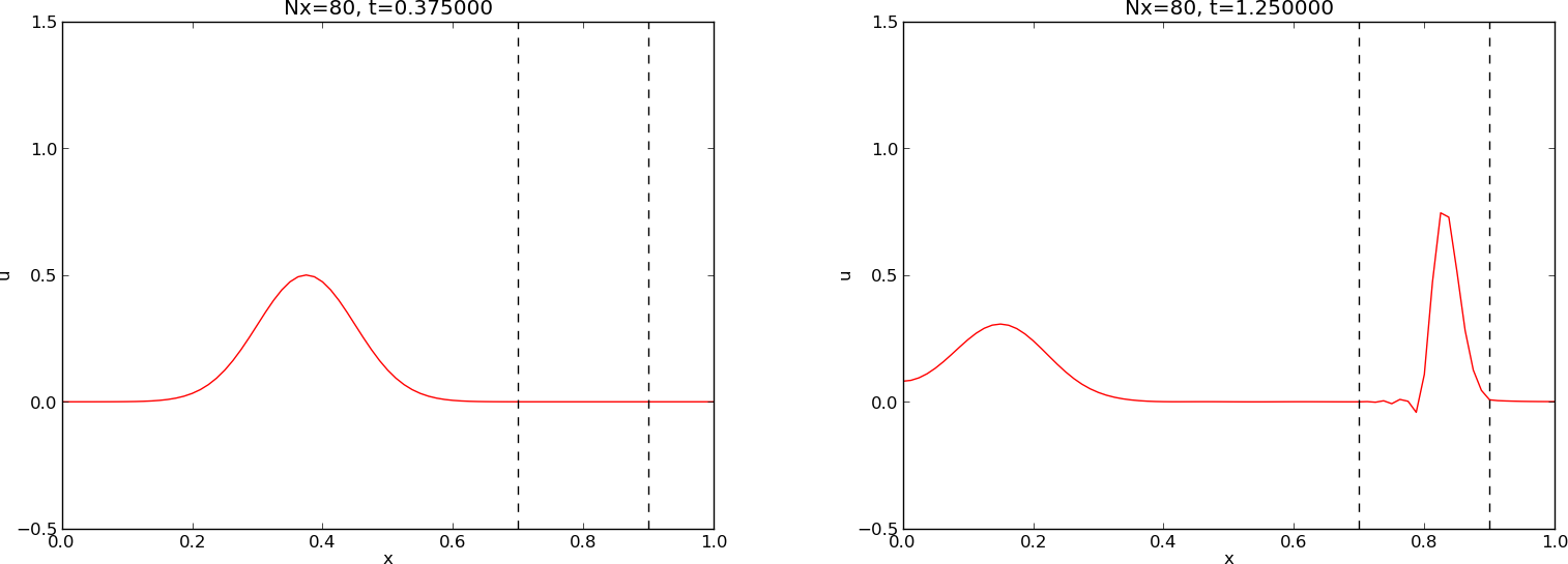
Our next generalization of the 1D wave equation (2.1) or (2.12) is to allow for a variable wave velocity \(c\): \(c=c(x)\), usually motivated by wave motion in a domain composed of different physical media. When the media differ in physical properties like density or porosity, the wave velocity \(c\) is affected and will depend on the position in space. Figure Figure 2.4 shows a wave propagating in one medium \([0, 0.7]\cup [0.9,1]\) with wave velocity \(c_1\) (left) before it enters a second medium \((0.7,0.9)\) with wave velocity \(c_2\) (right). When the wave meets the boundary where \(c\) jumps from \(c_1\) to \(c_2\), a part of the wave is reflected back into the first medium (the reflected wave), while one part is transmitted through the second medium (the transmitted wave).

Figure 2.4: Left: wave entering another medium; right: transmitted and reflected wave.

2.22 The model PDE with a variable coefficient

Instead of working with the squared quantity \(c^2(x)\), we shall for notational convenience introduce \(q(x) = c^2(x)\). A 1D wave equation with variable wave velocity often takes the form \[ \frac{\partial^2 u}{\partial t^2} = \frac{\partial}{\partial x}\left( q(x) \frac{\partial u}{\partial x}\right) + f(x,t) \tp \tag{2.30}\] This is the most frequent form of a wave equation with variable wave velocity, but other forms also appear, see Section Section 2.52 and equation (2.86).

As usual, we sample (2.30) at a mesh point, \[ \frac{\partial^2 }{\partial t^2} u(x_i,t_n) = \frac{\partial}{\partial x}\left( q(x_i) \frac{\partial}{\partial x} u(x_i,t_n)\right) + f(x_i,t_n), \] where the only new term to discretize is \[ \frac{\partial}{\partial x}\left( q(x_i) \frac{\partial}{\partial x} u(x_i,t_n)\right) = \left[ \frac{\partial}{\partial x}\left( q(x) \frac{\partial u}{\partial x}\right)\right]^n_i \tp \] ## Discretizing the variable coefficient {#sec-wave-pde2-var-c-ideas}

The principal idea is to first discretize the outer derivative. Define \[ \phi = q(x) \frac{\partial u}{\partial x}, \] and use a centered derivative around \(x=x_i\) for the derivative of \(\phi\): \[ \left[\frac{\partial\phi}{\partial x}\right]^n_i \approx \frac{\phi_{i+\half} - \phi_{i-\half}}{\Delta x} = [D_x\phi]^n_i \tp \] Then discretize \[ \phi_{i+\half} = q_{i+\half} \left[\frac{\partial u}{\partial x}\right]^n_{i+\half} \approx q_{i+\half} \frac{u^n_{i+1} - u^n_{i}}{\Delta x} = [q D_x u]_{i+\half}^n \tp \] Similarly, \[ \phi_{i-\half} = q_{i-\half} \left[\frac{\partial u}{\partial x}\right]^n_{i-\half} \approx q_{i-\half} \frac{u^n_{i} - u^n_{i-1}}{\Delta x} = [q D_x u]_{i-\half}^n \tp \] These intermediate results are now combined to \[ \left[ \frac{\partial}{\partial x}\left( q(x) \frac{\partial u}{\partial x}\right)\right]^n_i \approx \frac{1}{\Delta x^2} \left( q_{i+\half} \left({u^n_{i+1} - u^n_{i}}\right) - q_{i-\half} \left({u^n_{i} - u^n_{i-1}}\right)\right) \tp \tag{2.31}\] With operator notation we can write the discretization as \[ \left[ \frac{\partial}{\partial x}\left( q(x) \frac{\partial u}{\partial x}\right)\right]^n_i \approx [D_x (\overline{q}^{x} D_x u)]^n_i \tp \tag{2.32}\]

Do not use the chain rule on the spatial derivative term!

Many are tempted to use the chain rule on the term \(\frac{\partial}{\partial x}\left( q(x) \frac{\partial u}{\partial x}\right)\), but this is not a good idea when discretizing such a term.

The term with a variable coefficient expresses the net flux \(qu_x\) into a small volume (i.e., interval in 1D): \[ \frac{\partial}{\partial x}\left( q(x) \frac{\partial u}{\partial x}\right) \approx \frac{1}{\Delta x}(q(x+\Delta x)u_x(x+\Delta x) - q(x)u_x(x))\tp \] Our discretization reflects this principle directly: \(qu_x\) at the right end of the cell minus \(qu_x\) at the left end, because this follows from the formula (2.31) or \([D_x(q D_x u)]^n_i\).

When using the chain rule, we get two terms \(qu_{xx} + q_xu_x\). The typical discretization is \[ [D_x q D_x u + D_{2x}q D_{2x} u]_i^n, \tag{2.33}\] Writing this out shows that it is different from \([D_x(q D_x u)]^n_i\) and lacks the physical interpretation of net flux into a cell. With a smooth and slowly varying \(q(x)\) the differences between the two discretizations are not substantial. However, when \(q\) exhibits (potentially large) jumps, \([D_x(q D_x u)]^n_i\) with harmonic averaging of \(q\) yields a better solution than arithmetic averaging or (2.33). In the literature, the discretization \([D_x(q D_x u)]^n_i\) totally dominates and very few mention the alternative in (2.33).

2.23 Computing the coefficient between mesh points

If \(q\) is a known function of \(x\), we can easily evaluate \(q_{i+\half}\) simply as \(q(x_{i+\half})\) with \(x_{i+\half} = x_i + \half\Delta x\). However, in many cases \(c\), and hence \(q\), is only known as a discrete function, often at the mesh points \(x_i\). Evaluating \(q\) between two mesh points \(x_i\) and \(x_{i+1}\) must then be done by interpolation techniques, of which three are of particular interest in this context:

\[\begin{alignat}{2} q_{i+\half} &\approx \half\left( q_{i} + q_{i+1}\right) = [\overline{q}^{x}]_i \quad &\text{(arithmetic mean)} \\ q_{i+\half} &\approx 2\left( \frac{1}{q_{i}} + \frac{1}{q_{i+1}}\right)^{-1} \quad &\text{(harmonic mean)} \\ q_{i+\half} &\approx \left(q_{i}q_{i+1}\right)^{1/2} \quad &\text{(geometric mean)} \end{alignat}\]

The arithmetic mean is by far the most commonly used averaging technique and is well suited for smooth \(q(x)\) functions. The harmonic mean is often preferred when \(q(x)\) exhibits large jumps (which is typical for geological media). The geometric mean is less used, but popular in discretizations to linearize quadratic nonlinearities.

With the operator notation for the arithmetic mean we can specify the discretization of the complete variable-coefficient wave equation in a compact way: \[ \lbrack D_tD_t u = D_x\overline{q}^{x}D_x u + f\rbrack^{n}_i \tp \tag{2.34}\] Strictly speaking, \(\lbrack D_x\overline{q}^{x}D_x u\rbrack^{n}_i = \lbrack D_x (\overline{q}^{x}D_x u)\rbrack^{n}_i\).

From the compact difference notation we immediately see what kind of differences that each term is approximated with. The notation \(\overline{q}^{x}\) also specifies that the variable coefficient is approximated by an arithmetic mean, the definition being \([\overline{q}^{x}]_{i+\half}=(q_i+q_{i+1})/2\).

Before implementing, it remains to solve (2.34) with respect to \(u_i^{n+1}\):

\[ \begin{split} u^{n+1}_i = & - u_i^{n-1} + 2u_i^n + \\ &\quad \left(\frac{\Delta t}{\Delta x}\right)^2 \left( \half(q_{i} + q_{i+1})(u_{i+1}^n - u_{i}^n) - \half(q_{i} + q_{i-1})(u_{i}^n - u_{i-1}^n)\right) + \\ & \quad \Delta t^2 f^n_i \tp \end{split} \tag{2.35}\]

2.24 How a variable coefficient affects the stability

The stability criterion derived later (Section Section 2.42) reads \(\Delta t\leq \Delta x/c\). If \(c=c(x)\), the criterion will depend on the spatial location. We must therefore choose a \(\Delta t\) that is small enough such that no mesh cell has \(\Delta t > \Delta x/c(x)\). That is, we must use the largest \(c\) value in the criterion: \[ \Delta t \leq \beta \frac{\Delta x}{\max_{x\in [0,L]}c(x)} \tp \] The parameter \(\beta\) is included as a safety factor: in some problems with a significantly varying \(c\) it turns out that one must choose \(\beta <1\) to have stable solutions (\(\beta =0.9\) may act as an all-round value).

A different strategy to handle the stability criterion with variable wave velocity is to use a spatially varying \(\Delta t\). While the idea is mathematically attractive at first sight, the implementation quickly becomes very complicated, so we stick to a constant \(\Delta t\) and a worst case value of \(c(x)\) (with a safety factor \(\beta\)).

2.25 Neumann condition and a variable coefficient

Consider a Neumann condition \(\partial u/\partial x=0\) at \(x=L=N_x\Delta x\), discretized as \[ [D_{2x} u]^n_i = \frac{u_{i+1}^{n} - u_{i-1}^n}{2\Delta x} = 0\quad\Rightarrow\quad u_{i+1}^n = u_{i-1}^n, \] for \(i=N_x\). Using the scheme (2.35) at the end point \(i=N_x\) with \(u_{i+1}^n=u_{i-1}^n\) results in

\[ \begin{split} u^{n+1}_i &= - u_i^{n-1} + 2u_i^n + \\ &\quad \left(\frac{\Delta t}{\Delta x}\right)^2 \left( q_{i+\half}(u_{i-1}^n - u_{i}^n) - q_{i-\half}(u_{i}^n - u_{i-1}^n)\right) + \Delta t^2 f^n_i\\ &= - u_i^{n-1} + 2u_i^n + \left(\frac{\Delta t}{\Delta x}\right)^2 (q_{i+\half} + q_{i-\half})(u_{i-1}^n - u_{i}^n) + \Delta t^2 f^n_i \\ &\approx - u_i^{n-1} + 2u_i^n + \left(\frac{\Delta t}{\Delta x}\right)^2 2q_{i}(u_{i-1}^n - u_{i}^n) + \Delta t^2 f^n_i \tp \end{split} \tag{2.36}\] Here we used the approximation

\[\begin{align} q_{i+\half} + q_{i-\half} &= q_i + \left(\frac{dq}{dx}\right)_i \Delta x + \left(\frac{d^2q}{dx^2}\right)_i \Delta x^2 + \cdots +\nonumber\\ &\quad q_i - \left(\frac{dq}{dx}\right)_i \Delta x + \left(\frac{d^2q}{dx^2}\right)_i \Delta x^2 + \cdots\nonumber\\ &= 2q_i + 2\left(\frac{d^2q}{dx^2}\right)_i \Delta x^2 + \Oof{\Delta x^4} \nonumber\\ &\approx 2q_i \end{align}\]

An alternative derivation may apply the arithmetic mean of \(q_{n-\half}\) and \(q_{n+\half}\) in (2.36), leading to the term \[ (q_i + \half(q_{i+1}+q_{i-1}))(u_{i-1}^n-u_i^n)\tp \] Since \(\half(q_{i+1}+q_{i-1}) = q_i + \Oof{\Delta x^2}\), we can approximate with \(2q_i(u_{i-1}^n-u_i^n)\) for \(i=N_x\) and get the same term as we did above.

A common technique when implementing \(\partial u/\partial x=0\) boundary conditions, is to assume \(dq/dx=0\) as well. This implies \(q_{i+1}=q_{i-1}\) and \(q_{i+1/2}=q_{i-1/2}\) for \(i=N_x\). The implications for the scheme are

\[ \begin{split} u^{n+1}_i &= - u_i^{n-1} + 2u_i^n + \\ &\quad \left(\frac{\Delta t}{\Delta x}\right)^2 \left( q_{i+\half}(u_{i-1}^n - u_{i}^n) - q_{i-\half}(u_{i}^n - u_{i-1}^n)\right) + \\ & \quad \Delta t^2 f^n_i\\ &= - u_i^{n-1} + 2u_i^n + \left(\frac{\Delta t}{\Delta x}\right)^2 2q_{i-\half}(u_{i-1}^n - u_{i}^n) + \Delta t^2 f^n_i \tp \end{split} \tag{2.37}\]

2.26 Implementation of variable coefficients

The implementation of the scheme with a variable wave velocity \(q(x)=c^2(x)\) may assume that \(q\) is available as an array q[i] at the spatial mesh points. The following loop is a straightforward implementation of the scheme (2.35):

for i in range(1, Nx):
    u[i] = - u_nm1[i] + 2*u_n[i] + \
           C2*(0.5*(q[i] + q[i+1])*(u_n[i+1] - u_n[i])  - \
               0.5*(q[i] + q[i-1])*(u_n[i] - u_n[i-1])) + \
           dt2*f(x[i], t[n])

The coefficient C2 is now defined as (dt/dx)**2, i.e., not as the squared Courant number, since the wave velocity is variable and appears inside the parenthesis.

With Neumann conditions \(u_x=0\) at the boundary, we need to combine this scheme with the discrete version of the boundary condition, as shown in Section Section 2.25. Nevertheless, it would be convenient to reuse the formula for the interior points and just modify the indices ip1=i+1 and im1=i-1 as we did in Section Section 2.17. Assuming \(dq/dx=0\) at the boundaries, we can implement the scheme at the boundary with the following code.

i = 0
ip1 = i+1
im1 = ip1
u[i] = - u_nm1[i] + 2*u_n[i] + \
       C2*(0.5*(q[i] + q[ip1])*(u_n[ip1] - u_n[i])  - \
           0.5*(q[i] + q[im1])*(u_n[i] - u_n[im1])) + \
       dt2*f(x[i], t[n])

With ghost cells we can just reuse the formula for the interior points also at the boundary, provided that the ghost values of both \(u\) and \(q\) are correctly updated to ensure \(u_x=0\) and \(q_x=0\).

A vectorized version of the scheme with a variable coefficient at internal mesh points becomes

u[1:-1] = - u_nm1[1:-1] + 2*u_n[1:-1] + \
          C2*(0.5*(q[1:-1] + q[2:])*(u_n[2:] - u_n[1:-1]) -
              0.5*(q[1:-1] + q[:-2])*(u_n[1:-1] - u_n[:-2])) + \
          dt2*f(x[1:-1], t[n])

2.27 A more general PDE model with variable coefficients

Sometimes a wave PDE has a variable coefficient in front of the time-derivative term: \[ \varrho(x)\frac{\partial^2 u}{\partial t^2} = \frac{\partial}{\partial x}\left( q(x) \frac{\partial u}{\partial x}\right) + f(x,t) \tp \tag{2.38}\] One example appears when modeling elastic waves in a rod with varying density, cf.~(Section 2.52) with \(\varrho (x)\).

A natural scheme for (2.38) is \[ [\varrho D_tD_t u = D_x\overline{q}^xD_x u + f]^n_i \tp \] We realize that the \(\varrho\) coefficient poses no particular difficulty, since \(\varrho\) enters the formula just as a simple factor in front of a derivative. There is hence no need for any averaging of \(\varrho\). Often, \(\varrho\) will be moved to the right-hand side, also without any difficulty: \[ [D_tD_t u = \varrho^{-1}D_x\overline{q}^xD_x u + f]^n_i \tp \] ## Generalization: damping

Waves die out by two mechanisms. In 2D and 3D the energy of the wave spreads out in space, and energy conservation then requires the amplitude to decrease. This effect is not present in 1D. Damping is another cause of amplitude reduction. For example, the vibrations of a string die out because of damping due to air resistance and non-elastic effects in the string.

The simplest way of including damping is to add a first-order derivative to the equation (in the same way as friction forces enter a vibrating mechanical system): \[ \frac{\partial^2 u}{\partial t^2} + b\frac{\partial u}{\partial t} = c^2\frac{\partial^2 u}{\partial x^2} - f(x,t), \tag{2.39}\] where \(b \geq 0\) is a prescribed damping coefficient.

A typical discretization of (2.39) in terms of centered differences reads \[ [D_tD_t u + bD_{2t}u = c^2D_xD_x u + f]^n_i \tp \tag{2.40}\] Writing out the equation and solving for the unknown \(u^{n+1}_i\) gives the scheme \[ u^{n+1}_i = (1 + {\half}b\Delta t)^{-1}(({\half}b\Delta t -1) u^{n-1}_i + 2u^n_i + C^2 \left(u^{n}_{i+1}-2u^{n}_{i} + u^{n}_{i-1}\right) + \Delta t^2 f^n_i), \tag{2.41}\] for \(i\in\seti{\Ix}\) and \(n\geq 1\). New equations must be derived for \(u^1_i\), and for boundary points in case of Neumann conditions.

The damping is very small in many wave phenomena and thus only evident for very long time simulations. This makes the standard wave equation without damping relevant for a lot of applications.

2.28 Building a general 1D wave equation solver

A general 1D wave propagation solver targets the following initial-boundary value problem

\[ u_{tt} = (c^2(x)u_x)_x + f(x,t),\quad x\in (0,L),\ t\in (0,T] \tag{2.42}\] \[ u(x,0) = I(x),\quad x\in [0,L] \] \[ u_t(x,0) = V(t),\quad x\in [0,L] \] \[ u(0,t) = U_0(t)\text{ or } u_x(0,t)=0,\quad t\in (0,T] \] \[ u(L,t) = U_L(t)\text{ or } u_x(L,t)=0,\quad t\in (0,T] \]

The only new feature here is the time-dependent Dirichlet conditions, but they are trivial to implement:

i = Ix[0]  # x=0
u[i] = U_0(t[n+1])

i = Ix[-1] # x=L
u[i] = U_L(t[n+1])

For the Devito implementation of the 1D wave equation with general boundary conditions and variable wave velocity, see Section 2.12. The Devito solver extends the basic solver with:

• Neumann boundary conditions (\(u_x=0\))
• Time-varying Dirichlet conditions
• Variable wave velocity \(c(x)\)

The following sections explain various more advanced programming techniques for wave equation solvers.

2.29 User action function as a class

When building flexible solvers, it is useful to implement the callback function for visualization and data storage as a class. This provides a clean way to store state needed between calls.

2.29.1 The code

A class for flexible plotting, cleaning up files, and making movie files can be coded as follows:

class PlotAndStoreSolution:
    """
    Class for the user_action function in solver.
    Visualizes the solution only.
    """
    def __init__(
        self,
        casename='tmp',    # Prefix in filenames
        umin=-1, umax=1,   # Fixed range of y axis
        pause_between_frames=None,  # Movie speed
        screen_movie=True, # Show movie on screen?
        title='',          # Extra message in title
        skip_frame=1,      # Skip every skip_frame frame
        filename=None):    # Name of file with solutions
        self.casename = casename
        self.yaxis = [umin, umax]
        self.pause = pause_between_frames
        import matplotlib.pyplot as plt
        self.plt = plt
        self.screen_movie = screen_movie
        self.title = title
        self.skip_frame = skip_frame
        self.filename = filename
        if filename is not None:
            self.t = []
            filenames = glob.glob('.' + self.filename + '*.dat.npz')
            for filename in filenames:
                os.remove(filename)

        for filename in glob.glob('frame_*.png'):
            os.remove(filename)

    def __call__(self, u, x, t, n):
        """
        Callback function user_action, call by solver:
        Store solution, plot on screen and save to file.
        """
        if self.filename is not None:
            name = 'u%04d' % n  # array name
            kwargs = {name: u}
            fname = '.' + self.filename + '_' + name + '.dat'
            np.savez(fname, **kwargs)
            self.t.append(t[n])  # store corresponding time value
            if n == 0:           # save x once
                np.savez('.' + self.filename + '_x.dat', x=x)

        if n % self.skip_frame != 0:
            return
        title = 't=%.3f' % t[n]
        if self.title:
            title = self.title + ' ' + title

        if n == 0:
            self.plt.ion()
            self.lines = self.plt.plot(x, u, 'r-')
            self.plt.axis([x[0], x[-1],
                           self.yaxis[0], self.yaxis[1]])
            self.plt.xlabel('x')
            self.plt.ylabel('u')
            self.plt.title(title)
            self.plt.legend(['t=%.3f' % t[n]])
        else:
            self.lines[0].set_ydata(u)
            self.plt.legend(['t=%.3f' % t[n]])
            self.plt.draw()

        if t[n] == 0:
            time.sleep(2)  # let initial condition stay 2 s
        else:
            if self.pause is None:
                pause = 0.2 if u.size < 100 else 0
            time.sleep(pause)

        self.plt.savefig('frame_%04d.png' % (n))

2.29.2 Dissection

Understanding this class requires quite some familiarity with Python in general and class programming in particular. The class supports plotting with Matplotlib for visualization.

With the screen_movie parameter we can suppress displaying each movie frame on the screen. Alternatively, for slow movies associated with fine meshes, one can set skip_frame=10, causing every 10 frames to be shown.

The __call__ method makes PlotAndStoreSolution instances behave like functions, so we can just pass an instance, say p, as the user_action argument in the solver function, and any call to user_action will be a call to p.__call__. The __call__ method plots the solution on the screen, saves the plot to file, and stores the solution in a file for later retrieval.

More details on storing the solution in files appear in Section 11.4.

2.30 Pulse propagation in two media

Wave motion in heterogeneous media where \(c\) varies is an important application. One can specify an interval where the wave velocity is decreased by a factor (or increased by making this factor less than one). Figure Figure 2.4 shows a typical simulation scenario.

Four types of initial conditions are available:

1. a rectangular pulse (plug),
2. a Gaussian function (gaussian),
3. a “cosine hat” consisting of one period of the cosine function (cosinehat),
4. half a period of a “cosine hat” (half-cosinehat)

These peak-shaped initial conditions can be placed in the middle (loc='center') or at the left end (loc='left') of the domain. With the pulse in the middle, it splits in two parts, each with half the initial amplitude, traveling in opposite directions. With the pulse at the left end, centered at \(x=0\), and using the symmetry condition \(\partial u/\partial x=0\), only a right-going pulse is generated. There is also a left-going pulse, but it travels from \(x=0\) in negative \(x\) direction and is not visible in the domain \([0,L]\).

The pulse function is a flexible tool for playing around with various wave shapes and jumps in the wave velocity (i.e., discontinuous media). The code is shown to demonstrate how easy it is to reach this flexibility with the building blocks we have already developed:

def pulse(
    C=1,            # Maximum Courant number
    Nx=200,         # spatial resolution
    animate=True,
    version='vectorized',
    T=2,            # end time
    loc='left',     # location of initial condition
    pulse_tp='gaussian',  # pulse/init.cond. type
    slowness_factor=2, # inverse of wave vel. in right medium
    medium=[0.7, 0.9], # interval for right medium
    skip_frame=1,      # skip frames in animations
    sigma=0.05         # width measure of the pulse
    ):
    """
    Various peaked-shaped initial conditions on [0,1].
    Wave velocity is decreased by the slowness_factor inside
    medium. The loc parameter can be 'center' or 'left',
    depending on where the initial pulse is to be located.
    The sigma parameter governs the width of the pulse.
    """
    L = 1.0
    c_0 = 1.0
    if loc == 'center':
        xc = L/2
    elif loc == 'left':
        xc = 0

    if pulse_tp in ('gaussian','Gaussian'):
        def I(x):
            return np.exp(-0.5*((x-xc)/sigma)**2)
    elif pulse_tp == 'plug':
        def I(x):
            return 0 if abs(x-xc) > sigma else 1
    elif pulse_tp == 'cosinehat':
        def I(x):
            w = 2
            a = w*sigma
            return 0.5*(1 + np.cos(np.pi*(x-xc)/a)) \
                   if xc - a <= x <= xc + a else 0

    elif pulse_tp == 'half-cosinehat':
        def I(x):
            w = 4
            a = w*sigma
            return np.cos(np.pi*(x-xc)/a) \
                   if xc - 0.5*a <= x <= xc + 0.5*a else 0
    else:
        raise ValueError('Wrong pulse_tp="%s"' % pulse_tp)

    def c(x):
        return c_0/slowness_factor \
               if medium[0] <= x <= medium[1] else c_0

    umin=-0.5; umax=1.5*I(xc)
    casename = '%s_Nx%s_sf%s' % \
               (pulse_tp, Nx, slowness_factor)
    action = PlotMediumAndSolution(
        medium, casename=casename, umin=umin, umax=umax,
        skip_frame=skip_frame, screen_movie=animate,
        backend=None, filename='tmpdata')

    dt = (L/Nx)/c_0
    cpu, hashed_input = solver(
        I=I, V=None, f=None, c=c,
        U_0=None, U_L=None,
        L=L, dt=dt, C=C, T=T,
        user_action=action,
        version=version,
        stability_safety_factor=1)

    if cpu > 0:  # did we generate new data?
        action.close_file(hashed_input)
        action.make_movie_file()
    print('cpu (-1 means no new data generated):', cpu)

def convergence_rates(
    u_exact,
    I, V, f, c, U_0, U_L, L,
    dt0, num_meshes,
    C, T, version='scalar',
    stability_safety_factor=1.0):
    """
    Half the time step and estimate convergence rates for
    for num_meshes simulations.
    """
    class ComputeError:
        def __init__(self, norm_type):
            self.error = 0

        def __call__(self, u, x, t, n):
            """Store norm of the error in self.E."""
            error = np.abs(u - u_exact(x, t[n])).max()
            self.error = max(self.error, error)

    E = []
    h = []  # dt, solver adjusts dx such that C=dt*c/dx
    dt = dt0
    for i in range(num_meshes):
        error_calculator = ComputeError('Linf')
        solver(I, V, f, c, U_0, U_L, L, dt, C, T,
               user_action=error_calculator,
               version='scalar',
               stability_safety_factor=1.0)
        E.append(error_calculator.error)
        h.append(dt)
        dt /= 2  # halve the time step for next simulation
    print('E:', E)
    print('h:', h)
    r = [np.log(E[i]/E[i-1])/np.log(h[i]/h[i-1])
         for i in range(1,num_meshes)]
    return r

def test_convrate_sincos():
    n = m = 2
    L = 1.0
    u_exact = lambda x, t: np.cos(m*np.pi/L*t)*np.sin(m*np.pi/L*x)

    r = convergence_rates(
        u_exact=u_exact,
        I=lambda x: u_exact(x, 0),
        V=lambda x: 0,
        f=0,
        c=1,
        U_0=0,
        U_L=0,
        L=L,
        dt0=0.1,
        num_meshes=6,
        C=0.9,
        T=1,
        version='scalar',
        stability_safety_factor=1.0)
    print('rates sin(x)*cos(t) solution:',
          [round(r_,2) for r_ in r])
    assert abs(r[-1] - 2) < 0.002

The PlotMediumAndSolution class used here is a subclass of PlotAndStoreSolution where the medium with reduced \(c\) value, as specified by the medium interval, is visualized in the plots.

Comment on the choices of discretization parameters

The argument \(N_x\) in the pulse function does not correspond to the actual spatial resolution of \(C<1\), since the solver function takes a fixed \(\Delta t\) and \(C\), and adjusts \(\Delta x\) accordingly. As seen in the pulse function, the specified \(\Delta t\) is chosen according to the limit \(C=1\), so if \(C<1\), \(\Delta t\) remains the same, but the solver function operates with a larger \(\Delta x\) and smaller \(N_x\) than was specified in the call to pulse. The practical reason is that we always want to keep \(\Delta t\) fixed such that plot frames and movies are synchronized in time regardless of the value of \(C\) (i.e., \(\Delta x\) is varied when the Courant number varies).

The reader is encouraged to experiment with pulse propagation using the Devito solver from Section 2.12, which can be configured with different initial pulse shapes and variable wave velocities.

2.31 Exercise: Find the analytical solution to a damped wave equation

Consider the wave equation with damping (2.39). The goal is to find an exact solution to a wave problem with damping and zero source term. A starting point is the standing wave solution \(u = A \sin(k x) \cos(\omega t)\). It becomes necessary to include a damping term \(e^{-\beta t}\) and also have both a sine and cosine component in time: \[ u_{\text{e}}(x,t) = e^{-\beta t} \sin kx \left( A\cos\omega t - B\sin\omega t\right) \tp \] Find \(k\) from the boundary conditions \(u(0,t)=u(L,t)=0\). Then use the PDE to find constraints on \(\beta\), \(\omega\), \(A\), and \(B\). Set up a complete initial-boundary value problem and its solution.

Solution

Mathematical model: \[ \frac{\partial^2 u}{\partial t^2} + b\frac{\partial u}{\partial t} = c^2\frac{\partial^2 u}{\partial x^2}, \nonumber \] \(b \geq 0\) is a prescribed damping coefficient.

Ansatz: \[ u(x,t) = e^{-\beta t} \sin kx \left( A\cos\omega t - B\sin\omega t\right) \] Boundary condition: \(u=0\) for \(x=0,L\). Fulfilled for \(x=0\). Requirement at \(x=L\) gives \[ kL = m\pi, \] for an arbitrary integer \(m\). Hence, \(k=m\pi/L\).

Inserting the ansatz in the PDE and dividing by \(e^{-\beta t}\) results in

\[\begin{align*} (\beta^2 sin kx -\omega^2 sin kx - b\beta sin kx) (A\cos\omega t + B\sin\omega t) &+ \nonumber \\ (b\omega sin kx - 2\beta\omega sin kx) (-A\sin\omega t + B\cos\omega t) &= -(A\cos\omega t + B\sin\omega t)k^2c^2 \nonumber \end{align*}\]

This gives us two requirements: \[ \beta^2 - \omega^2 + b\beta + k^2c^2 = 0 \] and \[ -2\beta\omega + b\omega = 0 \] Since \(b\), \(c\) and \(k\) are to be given in advance, we may solve these two equations to get \[\begin{align*} \beta &= \frac{b}{2} \nonumber \\ \omega &= \sqrt{c^2k^2 - \frac{b^2}{4}} \nonumber \end{align*}\] From the initial condition on the derivative, i.e. \(\frac{\partial u_e}{\partial t} = 0\), we find that \[ B\omega = \beta A \] Inserting the expression for \(\omega\), we find that \[ B = \frac{b}{2\sqrt{c^2k^2 - \frac{b^2}{4}}} A \] for \(A\) prescribed.

Using \(t = 0\) in the expression for \(u_e\) gives us the initial condition as \[ I(x) = A sin kx \] Summarizing, the PDE problem can then be states as

\[\begin{align} \frac{\partial^2 u}{\partial t^2} + b\frac{\partial u}{\partial t} &= c^2 \frac{\partial^2 u}{\partial x^2}, \quad &x\in (0,L),\ t\in (0,T] \nonumber\\ u(x,0) &= I(x), \quad &x\in [0,L] \nonumber\\ \frac{\partial}{\partial t}u(x,0) &= 0, \quad &x\in [0,L] \nonumber\\ u(0,t) & = 0, \quad &t\in (0,T] \nonumber\\ u(L,t) & = 0, \quad &t\in (0,T] \nonumber \end{align}\] where constants \(c\), \(A\), \(b\) and \(k\), as well as \(I(x)\), are prescribed.

The solution to the problem is then given as \[ u_{\text{e}}(x,t) = e^{-\beta t} \sin kx \left( A\cos\omega t - B\sin\omega t\right) \tp \] with \(k=m\pi/L\) for arbitrary integer \(m\), \(\beta = \frac{b}{2}\), \(\omega = \sqrt{c^2k^2 - \frac{b^2}{4}}\), \(B = \frac{b}{2\sqrt{c^2k^2 - \frac{b^2}{4}}} A\) and \(I(x) = A sin kx\).

2.32 Problem: Explore symmetry boundary conditions

Consider the simple “plug” wave where \(\Omega = [-L,L]\) and \[ I(x) = \left\lbrace\begin{array}{ll} 1, & x\in [-\delta, \delta],\\ 0, & \text{otherwise} \end{array}\right. \] for some number \(0 < \delta < L\). The other initial condition is \(u_t(x,0)=0\) and there is no source term \(f\). The boundary conditions can be set to \(u=0\). The solution to this problem is symmetric around \(x=0\). This means that we can simulate the wave process in only half of the domain \([0,L]\).

a)

Argue why the symmetry boundary condition is \(u_x=0\) at \(x=0\).

Symmetry of a function about \(x=x_0\) means that

\(f(x_0+h) = f(x_0-h)\).

Solution

A symmetric \(u\) around \(x=0\) means that \(u(-x,t)=u(x,t)\). Let \(x_0=0\) and \(x=x_0+h\). Then we can use a centered finite difference definition of the derivative: \[ \frac{\partial}{\partial x}u(x_0,t) = \lim_{h\rightarrow 0}\frac{u(x_0+h,t)- u(x_0-h)}{2h} = \lim_{h\rightarrow 0}\frac{u(h,t)- u(-h,t)}{2h} = 0, \] since \(u(h,t)=u(-h,t)\) for any \(h\). Symmetry around a point \(x=x_0\) therefore always implies \(u_x(x_0,t)=0\).

b)

Perform simulations of the complete wave problem on \([-L,L]\). Thereafter, utilize the symmetry of the solution and run a simulation in half of the domain \([0,L]\), using a boundary condition at \(x=0\). Compare plots from the two solutions and confirm that they are the same.

Solution

The approach is to solve the two problems: on \([-L,L]\) with boundary conditions \(u(-L,t)=u(L,t)=0\), and on \([0,L]\) with boundary conditions \(u_x(0,t)=0\) and \(u(L,t)=0\). See Section 2.12 for the Devito implementation with Neumann boundary conditions.

The solutions from the two formulations should be identical, demonstrating the validity of the symmetry approach.

c)

Prove the symmetry property of the solution by setting up the complete initial-boundary value problem and showing that if \(u(x,t)\) is a solution, then also \(u(-x,t)\) is a solution.

Solution

The plan in this proof is to introduce \(v(x,t)=u(-x,t)\) and show that \(v\) fulfills the same initial-boundary value problem as \(u\). If the problem has a unique solution, then \(v=u\). Or, in other words, the solution is symmetric: \(u(-x,t)=u(x,t)\).

We can work with a general initial-boundary value problem on the form

\[\begin{align} u_tt(x,t) &= c^2u_{xx}(x,t) + f(x,t)\\ u(x,0) &= I(x)\\ u_t(x,0) &= V(x)\\ u(-L,0) &= 0\\ u(L,0) &= 0 \end{align}\] Introduce a new coordinate \(\bar x = -x\). We have that \[ \frac{\partial^2 u}{\partial x^2} = \frac{\partial}{\partial x} \left( \frac{\partial u}{\partial\bar x} \frac{\partial\bar x}{\partial x} \right) = \frac{\partial}{\partial x} \left( \frac{\partial u}{\partial\bar x} (-1)\right) = (-1)^2 \frac{\partial^2 u}{\partial \bar x^2} \] The derivatives in time are unchanged.

Substituting \(x\) by \(-\bar x\) leads to

\[\begin{align} u_{tt}(-\bar x,t) &= c^2u_{\bar x\bar x}(-\bar x,t) + f(-\bar x,t)\\ u(-\bar x,0) &= I(-\bar x)\\ u_t(-\bar x,0) &= V(-\bar x)\\ u(L,0) &= 0\\ u(-L,0) &= 0 \end{align}\] Now, dropping the bars and introducing \(v(x,t)=u(-x,t)\), we find that

\[\begin{align} v_{tt}(x,t) &= c^2v_{xx}(x,t) + f(-x,t)\\ v(x,0) &= I(-x)\\ v_t(x ,0) &= V(-x)\\ v(-L,0) &= 0\\ v(L,0) &= 0 \end{align}\] Provided that \(I\), \(f\), and \(V\) are all symmetric around \(x=0\) such that \(I(x)=I(-x)\), \(V(x)=V(-x)\), and \(f(x,t)=f(-x,t)\), we can express the initial-boundary value problem as

\[\begin{align} v_{tt}(x,t) &= c^2v_{xx}(x,t) + f(x,t)\\ v(x,0) &= I(x)\\ v_t(x ,0) &= V(x)\\ v(-L,0) &= 0\\ v(L,0) &= 0 \end{align}\] This is the same problem as the one that \(u\) fulfills. If the solution is unique, which can be proven, then \(v=u\), and \(u(-x,t)=u(x,t)\).

To summarize, the necessary conditions for symmetry are that

• all involved functions \(I\), \(V\), and \(f\) must be symmetric, and
• the boundary conditions are symmetric in the sense that they can be flipped (the condition at \(x=-L\) can be applied at \(x=L\) and vice versa).

d)

If the code works correctly, the solution \(u(x,t) = x(L-x)(1+\frac{t}{2})\) should be reproduced exactly. Write a test function test_quadratic that checks whether this is the case. Simulate for \(x\) in \([0, \frac{L}{2}]\) with a symmetry condition at the end \(x = \frac{L}{2}\).

Solution

Running the code below, shows that the test case indeed is reproduced exactly.

def test_quadratic():
    """
    Check the scalar and vectorized versions work for
    a quadratic u(x,t)=x(L-x)(1+t/2) that is exactly reproduced.
    We simulate in [0, L/2] and apply a symmetry condition
    at the end x=L/2.
    """
    exact_solution = lambda x, t: x * (L - x) * (1 + 0.5 * t)
    I = lambda x: exact_solution(x, 0)
    V = lambda x: 0.5 * exact_solution(x, 0)
    f = lambda x, t: 2 * (1 + 0.5 * t) * c**2
    U_0 = lambda t: exact_solution(0, t)
    U_L = None
    L = 2.5
    c = 1.5
    Nx = 3  # very coarse mesh
    C = 1
    T = 18  # long time integration

    def assert_no_error(u, x, t, n):
        u_e = exact_solution(x, t[n])
        diff = abs(u - u_e).max()
        assert diff < 1e-13, f"Max error: {diff}"

    solver(
        I, V, f, c, U_0, U_L, 0, L / 2, Nx, C, T,
        user_action=assert_no_error, version="scalar",
    )
    solver(
        I, V, f, c, U_0, U_L, 0, L / 2, Nx, C, T,
        user_action=assert_no_error, version="vectorized",
    )

2.33 Exercise: Send pulse waves through a layered medium

Investigate sending a pulse, located with its peak at \(x=0\), through two media with different wave velocities. The (scaled) velocity in the left medium is 1 while it is \(\frac{1}{s_f}\) in the right medium. Report what happens with a Gaussian pulse, a “cosine hat” pulse, half a “cosine hat” pulse, and a plug pulse for resolutions \(N_x=40,80,160\), and \(s_f=2,4\). Simulate until \(T=2\).

Use the Devito solver from Section 2.12 with variable wave velocity.

Solution

In all cases, the change in velocity causes some of the wave to be reflected back (while the rest is let through). When the waves go from higher to lower velocity, the amplitude builds, and vice versa.

2.34 Exercise: Explain why numerical noise occurs

The experiments performed in Exercise Section 2.33 shows considerable numerical noise in the form of non-physical waves, especially for \(s_f=4\) and the plug pulse or the half a “cosinehat” pulse. The noise is much less visible for a Gaussian pulse. Run the case with the plug and half a “cosinehat” pulse for \(s_f=1\), \(C=0.9, 0.25\), and \(N_x=40,80,160\). Use the numerical dispersion relation to explain the observations.

2.35 Exercise: Investigate harmonic averaging in a 1D model

Harmonic means are often used if the wave velocity is non-smooth or discontinuous. Will harmonic averaging of the wave velocity give less numerical noise for the case \(s_f=4\) in Exercise Section 2.33?

2.36 Problem: Implement open boundary conditions

To enable a wave to leave the computational domain and travel undisturbed through the boundary \(x=L\), one can in a one-dimensional problem impose the following condition, called a radiation condition or open boundary condition (Engquist and Majda 1977; Clayton and Engquist 1977): \[ \frac{\partial u}{\partial t} + c\frac{\partial u}{\partial x} = 0\tp \tag{2.43}\] The parameter \(c\) is the wave velocity. Higher-order absorbing boundary conditions (Higdon 1986) can handle oblique incidence in multiple dimensions; see Section 2.50 for a comprehensive treatment.

Show that (2.43) accepts a solution \(u = g_R(x-ct)\) (right-going wave), but not \(u = g_L(x+ct)\) (left-going wave). This means that (2.43) will allow any right-going wave \(g_R(x-ct)\) to pass through the boundary undisturbed.

A corresponding open boundary condition for a left-going wave through \(x=0\) is \[ \frac{\partial u}{\partial t} - c\frac{\partial u}{\partial x} = 0\tp \tag{2.44}\]

a)

A natural idea for discretizing the condition (2.43) at the spatial end point \(i=N_x\) is to apply centered differences in time and space: \[ [D_{2t}u + cD_{2x}u =0]^n_{i},\quad i=N_x\tp \tag{2.45}\] Eliminate the fictitious value \(u_{N_x+1}^n\) by using the discrete equation at the same point.

The equation for the first step, \(u_i^1\), is in principle also affected, but we can then use the condition \(u_{N_x}=0\) since the wave has not yet reached the right boundary.

b)

A much more convenient implementation of the open boundary condition at \(x=L\) can be based on an explicit discretization \[ [D^+_tu + cD_x^- u = 0]_i^n,\quad i=N_x\tp \tag{2.46}\] From this equation, one can solve for \(u^{n+1}_{N_x}\) and apply the formula as a Dirichlet condition at the boundary point. However, the finite difference approximations involved are of first order.

Implement this scheme for a wave equation \(u_{tt}=c^2u_{xx}\) in a domain \([0,L]\), where you have \(u_x=0\) at \(x=0\), the condition (2.43) at \(x=L\), and an initial disturbance in the middle of the domain, e.g., a plug profile like \[ u(x,0) = \left\lbrace\begin{array}{ll} 1,& L/2-\ell \leq x \leq L/2+\ell,\\ 0,\text{otherwise}\end{array}\right. \] Observe that the initial wave is split in two, the left-going wave is reflected at \(x=0\), and both waves travel out of \(x=L\), leaving the solution as \(u=0\) in \([0,L]\). Use a unit Courant number such that the numerical solution is exact. Make a movie to illustrate what happens.

Because this simplified implementation of the open boundary condition works, there is no need to pursue the more complicated discretization in a).

Hint

Modify the Devito solver from Section 2.12 to implement this condition.

c)

Add the possibility to have either \(u_x=0\) or an open boundary condition at the left boundary. The latter condition is discretized as \[ [D^+_tu - cD_x^+ u = 0]_i^n,\quad i=0, \tag{2.47}\] leading to an explicit update of the boundary value \(u^{n+1}_0\).

The implementation can be tested with a Gaussian function as initial condition: \[ g(x;m,s) = \frac{1}{\sqrt{2\pi}s}e^{-\frac{(x-m)^2}{2s^2}}\tp \] Run two tests:

1. Disturbance in the middle of the domain, \(I(x)=g(x;L/2,s)\), and open boundary condition at the left end.
2. Disturbance at the left end, \(I(x)=g(x;0,s)\), and \(u_x=0\) as symmetry boundary condition at this end.

Make test functions for both cases, testing that the solution is zero after the waves have left the domain.

d)

In 2D and 3D it is difficult to compute the correct wave velocity normal to the boundary, which is needed in generalizations of the open boundary conditions in higher dimensions. Test the effect of having a slightly wrong wave velocity in (2.46). Make movies to illustrate what happens.

Remarks

The condition (2.43) works perfectly in 1D when \(c\) is known. In 2D and 3D, however, the condition reads \(u_t + c_x u_x + c_y u_y=0\), where \(c_x\) and \(c_y\) are the wave speeds in the \(x\) and \(y\) directions. Estimating these components (i.e., the direction of the wave) is often challenging. Other methods are normally used in 2D and 3D to let waves move out of a computational domain.

2.37 Exercise: Implement periodic boundary conditions

It is frequently of interest to follow wave motion over large distances and long times. A straightforward approach is to work with a very large domain, but that might lead to a lot of computations in areas of the domain where the waves cannot be noticed. A more efficient approach is to let a right-going wave out of the domain and at the same time let it enter the domain on the left. This is called a periodic boundary condition.

The boundary condition at the right end \(x=L\) is an open boundary condition (see Exercise Section 2.36) to let a right-going wave out of the domain. At the left end, \(x=0\), we apply, in the beginning of the simulation, either a symmetry boundary condition (see Exercise Section 2.32) \(u_x=0\), or an open boundary condition.

This initial wave will split in two and either be reflected or transported out of the domain at \(x=0\). The purpose of the exercise is to follow the right-going wave. We can do that with a periodic boundary condition. This means that when the right-going wave hits the boundary \(x=L\), the open boundary condition lets the wave out of the domain, but at the same time we use a boundary condition on the left end \(x=0\) that feeds the outgoing wave into the domain again. This periodic condition is simply \(u(0)=u(L)\). The switch from \(u_x=0\) or an open boundary condition at the left end to a periodic condition can happen when \(u(L,t)>\epsilon\), where \(\epsilon =10^{-4}\) might be an appropriate value for determining when the right-going wave hits the boundary \(x=L\).

The open boundary conditions can conveniently be discretized as explained in Exercise Section 2.36. Implement the described type of boundary conditions and test them on two different initial shapes: a plug \(u(x,0)=1\) for \(x\leq 0.1\), \(u(x,0)=0\) for \(x>0.1\), and a Gaussian function in the middle of the domain: \(u(x,0)=\exp{(-\frac{1}{2}(x-0.5)^2/0.05)}\). The domain is the unit interval \([0,1]\). Run these two shapes for Courant numbers 1 and 0.5. Assume constant wave velocity. Make movies of the four cases. Reason why the solutions are correct.

2.38 Exercise: Compare discretizations of a Neumann condition

We have a 1D wave equation with variable wave velocity: \(u_{tt}=(qu_x)_x\). A Neumann condition \(u_x\) at \(x=0, L\) can be discretized as shown in (2.36) and (2.37).

The aim of this exercise is to examine the rate of the numerical error when using different ways of discretizing the Neumann condition.

a)

As a test problem, \(q=1+(x-L/2)^4\) can be used, with \(f(x,t)\) adapted such that the solution has a simple form, say \(u(x,t)=\cos (\pi x/L)\cos (\omega t)\) for, e.g., \(\omega = 1\). Perform numerical experiments and find the convergence rate of the error using the approximation (2.36).

b)

Switch to \(q(x)=1+\cos(\pi x/L)\), which is symmetric at \(x=0,L\), and check the convergence rate of the scheme (2.37). Now, \(q_{i-1/2}\) is a 2nd-order approximation to \(q_i\), \(q_{i-1/2}=q_i + 0.25q_i''\Delta x^2 + \cdots\), because \(q_i'=0\) for \(i=N_x\) (a similar argument can be applied to the case \(i=0\)).

c)

A third discretization can be based on a simple and convenient, but less accurate, one-sided difference: \(u_{i}-u_{i-1}=0\) at \(i=N_x\) and \(u_{i+1}-u_i=0\) at \(i=0\). Derive the resulting scheme in detail and implement it. Run experiments with \(q\) from a) or b) to establish the rate of convergence of the scheme.

d)

A fourth technique is to view the scheme as \[ [D_tD_tu]^n_i = \frac{1}{\Delta x}\left( [qD_xu]_{i+\half}^n - [qD_xu]_{i-\half}^n\right) - [f]_i^n, \] and place the boundary at \(x_{i+\half}\), \(i=N_x\), instead of exactly at the physical boundary. With this idea of approximating (moving) the boundary, we can just set \([qD_xu]_{i+\half}^n=0\). Derive the complete scheme using this technique. The implementation of the boundary condition at \(L-\Delta x/2\) is \(\Oof{\Delta x^2}\) accurate, but the interesting question is what impact the movement of the boundary has on the convergence rate. Compute the errors as usual over the entire mesh and use \(q\) from a) or b).

2.39 Exercise: Verification by a cubic polynomial in space

The purpose of this exercise is to verify the implementation of a wave equation solver using an exact numerical solution for the wave equation \(u_{tt}=c^2u_{xx} + f\) with Neumann boundary conditions \(u_x(0,t)=u_x(L,t)=0\). Use the Devito solver from Section 2.12.

The idea of verification using a quadratic polynomial is to produce a solution that is a lower-order polynomial such that both the PDE problem, the boundary conditions, and all the discrete equations are exactly fulfilled. Then the solver function should reproduce this exact solution to machine precision. More precisely, we seek \(u=X(x)T(t)\), with \(T(t)\) as a linear function and \(X(x)\) as a parabola that fulfills the boundary conditions. Inserting this \(u\) in the PDE determines \(f\). It turns out that \(u\) also fulfills the discrete equations, because the truncation error of the discretized PDE has derivatives in \(x\) and \(t\) of order four and higher. These derivatives all vanish for a quadratic \(X(x)\) and linear \(T(t)\).

It would be attractive to use a similar approach in the case of Neumann conditions. We set \(u=X(x)T(t)\) and seek lower-order polynomials \(X\) and \(T\). To force \(u_x\) to vanish at the boundary, we let \(X_x\) be a parabola. Then \(X\) is a cubic polynomial. The fourth-order derivative of a cubic polynomial vanishes, so \(u=X(x)T(t)\) will fulfill the discretized PDE also in this case, if \(f\) is adjusted such that \(u\) fulfills the PDE.

However, the discrete boundary condition is not exactly fulfilled by this choice of \(u\). The reason is that \[ [D_{2x}u]^n_i = u_{x}(x_i,t_n) + \frac{1}{6}u_{xxx}(x_i,t_n)\Delta x^2 - \Oof{\Delta x^4}\tp \tag{2.48}\] At the two boundary points, we must demand that the derivative \(X_x(x)=0\) such that \(u_x=0\). However, \(u_{xxx}\) is a constant and not zero when \(X(x)\) is a cubic polynomial. Therefore, our \(u=X(x)T(t)\) fulfills \[ [D_{2x}u]^n_i = \frac{1}{6}u_{xxx}(x_i,t_n)\Delta x^2, \] and not \[ [D_{2x}u]^n_i =0, \quad i=0,N_x, \] as it should. (Note that all the higher-order terms \(\Oof{\Delta x^4}\) also have higher-order derivatives that vanish for a cubic polynomial.) So to summarize, the fundamental problem is that \(u\) as a product of a cubic polynomial and a linear or quadratic polynomial in time is not an exact solution of the discrete boundary conditions.

To make progress, we assume that \(u=X(x)T(t)\), where \(T\) for simplicity is taken as a prescribed linear function \(1+\frac{1}{2}t\), and \(X(x)\) is taken as an unknown cubic polynomial \(\sum_{j=0}^3 a_jx^j\). There are two different ways of determining the coefficients \(a_0,\ldots,a_3\) such that both the discretized PDE and the discretized boundary conditions are fulfilled, under the constraint that we can specify a function \(f(x,t)\) for the PDE to feed to the solver function. Both approaches are explained in the subexercises.

a)

One can insert \(u\) in the discretized PDE and find the corresponding \(f\). Then one can insert \(u\) in the discretized boundary conditions. This yields two equations for the four coefficients \(a_0,\ldots,a_3\). To find the coefficients, one can set \(a_0=0\) and \(a_1=1\) for simplicity and then determine \(a_2\) and \(a_3\). This approach will make \(a_2\) and \(a_3\) depend on \(\Delta x\) and \(f\) will depend on both \(\Delta x\) and \(\Delta t\).

Use sympy to perform analytical computations. A starting point is to define \(u\) as follows:

def test_cubic1():
    import sympy as sm
    x, t, c, L, dx, dt = sm.symbols('x t c L dx dt')
    i, n = sm.symbols('i n', integer=True)

    T = lambda t: 1 + sm.Rational(1,2)*t  # Temporal term
    a = sm.symbols('a_0 a_1 a_2 a_3')
    X = lambda x: sum(a[q]*x**q for q in range(4))  # Spatial term
    u = lambda x, t: X(x)*T(t)

The symbolic expression for \(u\) is reached by calling u(x,t) with x and t as sympy symbols.

Define DxDx(u, i, n), DtDt(u, i, n), and D2x(u, i, n) as Python functions for returning the difference approximations \([D_xD_x u]^n_i\), \([D_tD_t u]^n_i\), and \([D_{2x}u]^n_i\). The next step is to set up the residuals for the equations \([D_{2x}u]^n_0=0\) and \([D_{2x}u]^n_{N_x}=0\), where \(N_x=L/\Delta x\). Call the residuals R_0 and R_L. Substitute \(a_0\) and \(a_1\) by 0 and 1, respectively, in R_0, R_L, and a:

R_0 = R_0.subs(a[0], 0).subs(a[1], 1)
R_L = R_L.subs(a[0], 0).subs(a[1], 1)
a = list(a)  # enable in-place assignment
a[0:2] = 0, 1

Determining \(a_2\) and \(a_3\) from the discretized boundary conditions is then about solving two equations with respect to \(a_2\) and \(a_3\), i.e., a[2:]:

s = sm.solve([R_0, R_L], a[2:])
a[2:] = s[a[2]], s[a[3]]

Now, a contains computed values and u will automatically use these new values since X accesses a.

Compute the source term \(f\) from the discretized PDE: \(f^n_i = [D_tD_t u - c^2D_xD_x u]^n_i\). Turn \(u\), the time derivative \(u_t\) (needed for the initial condition \(V(x)\)), and \(f\) into Python functions. Set numerical values for \(L\), \(N_x\), \(C\), and \(c\). Prescribe the time interval as \(\Delta t = CL/(N_xc)\), which imply \(\Delta x = c\Delta t/C = L/N_x\). Define new functions I(x), V(x), and f(x,t) as wrappers of the ones made above, where fixed values of \(L\), \(c\), \(\Delta x\), and \(\Delta t\) are inserted, such that I, V, and f can be passed on to the solver function. Finally, call solver with a user_action function that compares the numerical solution to this exact solution \(u\) of the discrete PDE problem.

To turn a sympy expression e, depending on a series of

symbols, say x, t, dx, dt, L, and c, into a plain Python function e_exact(x,t,L,dx,dt,c), one can write

e_exact = sm.lambdify([x,t,L,dx,dt,c], e, 'numpy')

The 'numpy' argument is a good habit as the e_exact function will then work with array arguments if it contains mathematical functions (but here we only do plain arithmetics, which automatically work with arrays).

b)

An alternative way of determining \(a_0,\ldots,a_3\) is to reason as follows. We first construct \(X(x)\) such that the boundary conditions are fulfilled: \(X=x(L-x)\). However, to compensate for the fact that this choice of \(X\) does not fulfill the discrete boundary condition, we seek \(u\) such that \[ u_x = \frac{\partial}{\partial x}x(L-x)T(t) - \frac{1}{6}u_{xxx}\Delta x^2, \] since this \(u\) will fit the discrete boundary condition. Assuming \(u=T(t)\sum_{j=0}^3a_jx^j\), we can use the above equation to determine the coefficients \(a_1,a_2,a_3\). A value, e.g., 1 can be used for \(a_0\). The following sympy code computes this \(u\):

def test_cubic2():
    import sympy as sm
    x, t, c, L, dx = sm.symbols('x t c L dx')
    T = lambda t: 1 + sm.Rational(1,2)*t  # Temporal term
    X = lambda x: sum(a[i]*x**i for i in range(4))
    a = sm.symbols('a_0 a_1 a_2 a_3')
    u = lambda x, t: X(x)*T(t)
    R = sm.diff(u(x,t), x) - (
        x*(L-x) - sm.Rational(1,6)*sm.diff(u(x,t), x, x, x)*dx**2)
    R = sm.poly(R, x)
    coeff = R.all_coeffs()
    s = sm.solve(coeff, a[1:])  # a[0] is not present in R
    s[a[0]] = 1
    X = lambda x: sm.simplify(sum(s[a[i]]*x**i for i in range(4)))
    u = lambda x, t: X(x)*T(t)
    print 'u:', u(x,t)

The next step is to find the source term f_e by inserting u_e in the PDE. Thereafter, turn u, f, and the time derivative of u into plain Python functions as in a), and then wrap these functions in new functions I, V, and f, with the right signature as required by the solver function. Set parameters as in a) and check that the solution is exact to machine precision at each time level using an appropriate user_action function.

2.40 Analysis of the wave equation

2.40.1 Properties of the solution

The wave equation \[ \frac{\partial^2 u}{\partial t^2} = c^2 \frac{\partial^2 u}{\partial x^2} \] has solutions of the form \[ u(x,t) = g_R(x-ct) + g_L(x+ct), \tag{2.49}\] for any functions \(g_R\) and \(g_L\) sufficiently smooth to be differentiated twice. The result follows from inserting (2.49) in the wave equation. A function of the form \(g_R(x-ct)\) represents a signal moving to the right in time with constant velocity \(c\). This feature can be explained as follows. At time \(t=0\) the signal looks like \(g_R(x)\). Introducing a moving horizontal coordinate \(\xi = x-ct\), we see the function \(g_R(\xi)\) is “at rest” in the \(\xi\) coordinate system, and the shape is always the same. Say the \(g_R(\xi)\) function has a peak at \(\xi=0\). This peak is located at \(x=ct\), which means that it moves with the velocity \(dx/dt=c\) in the \(x\) coordinate system. Similarly, \(g_L(x+ct)\) is a function, initially with shape \(g_L(x)\), that moves in the negative \(x\) direction with constant velocity \(c\) (introduce \(\xi=x+ct\), look at the point \(\xi=0\), \(x=-ct\), which has velocity \(dx/dt=-c\)).

With the particular initial conditions \[ u(x,0)=I(x),\quad \frac{\partial}{\partial t}u(x,0) =0, \] we get, with \(u\) as in (2.49), \[ g_R(x) + g_L(x) = I(x),\quad -cg_R'(x) + cg_L'(x) = 0\tp \] The former suggests \(g_R=g_L\), and the former then leads to \(g_R=g_L=I/2\). Consequently, \[ u(x,t) = \half I(x-ct) + \half I(x+ct) \tp \tag{2.50}\] The interpretation of (2.50) is that the initial shape of \(u\) is split into two parts, each with the same shape as \(I\) but half of the initial amplitude. One part is traveling to the left and the other one to the right.

The solution has two important physical features: constant amplitude of the left and right wave, and constant velocity of these two waves. It turns out that the numerical solution will also preserve the constant amplitude, but the velocity depends on the mesh parameters \(\Delta t\) and \(\Delta x\).

The solution (2.50) will be influenced by boundary conditions when the parts \(\half I(x-ct)\) and \(\half I(x+ct)\) hit the boundaries and get, e.g., reflected back into the domain. However, when \(I(x)\) is nonzero only in a small part in the middle of the spatial domain \([0,L]\), which means that the boundaries are placed far away from the initial disturbance of \(u\), the solution (2.50) is very clearly observed in a simulation.

A useful representation of solutions of wave equations is a linear combination of sine and/or cosine waves. Such a sum of waves is a solution if the governing PDE is linear and each sine or cosine wave fulfills the equation. To ease analytical calculations by hand we shall work with complex exponential functions instead of real-valued sine or cosine functions. The real part of complex expressions will typically be taken as the physical relevant quantity (whenever a physical relevant quantity is strictly needed). The idea now is to build \(I(x)\) of complex wave components \(e^{ikx}\): \[ I(x) \approx \sum_{k\in K} b_k e^{ikx} \tp \tag{2.51}\] Here, \(k\) is the frequency of a component, \(K\) is some set of all the discrete \(k\) values needed to approximate \(I(x)\) well, and \(b_k\) are constants that must be determined. We will very seldom need to compute the \(b_k\) coefficients: most of the insight we look for, and the understanding of the numerical methods we want to establish, come from investigating how the PDE and the scheme treat a single component \(e^{ikx}\) wave.

Letting the number of \(k\) values in \(K\) tend to infinity, makes the sum (2.51) converge to \(I(x)\). This sum is known as a Fourier series representation of \(I(x)\). Looking at (2.50), we see that the solution \(u(x,t)\), when \(I(x)\) is represented as in (2.51), is also built of basic complex exponential wave components of the form \(e^{ik(x\pm ct)}\) according to \[ u(x,t) = \half \sum_{k\in K} b_k e^{ik(x - ct)} + \half \sum_{k\in K} b_k e^{ik(x + ct)} \tp \tag{2.52}\] It is common to introduce the frequency in time \(\omega = kc\) and assume that \(u(x,t)\) is a sum of basic wave components written as \(e^{ikx -\omega t}\). (Observe that inserting such a wave component in the governing PDE reveals that \(\omega^2 = k^2c^2\), or \(\omega =\pm kc\), reflecting the two solutions: one (\(+kc\)) traveling to the right and the other (\(-kc\)) traveling to the left.)

2.41 More precise definition of Fourier representations

The above introduction to function representation by sine and cosine waves was quick and intuitive, but will suffice as background knowledge for the following material of single wave component analysis. However, to understand all details of how different wave components sum up to the analytical and numerical solutions, a more precise mathematical treatment is helpful and therefore summarized below.

It is well known that periodic functions can be represented by Fourier series. A generalization of the Fourier series idea to non-periodic functions defined on the real line is the Fourier transform:

\[ I(x) = \int_{-\infty}^\infty A(k)e^{ikx}dk, \tag{2.53}\] \[ A(k) = \int_{-\infty}^\infty I(x)e^{-ikx}dx\tp \tag{2.54}\] The function \(A(k)\) reflects the weight of each wave component \(e^{ikx}\) in an infinite sum of such wave components. That is, \(A(k)\) reflects the frequency content in the function \(I(x)\). Fourier transforms are particularly fundamental for analyzing and understanding time-varying signals.

The solution of the linear 1D wave PDE can be expressed as \[ u(x,t) = \int_{-\infty}^\infty A(k)e^{i(kx-\omega(k)t)}dx\tp \] In a finite difference method, we represent \(u\) by a mesh function \(u^n_q\), where \(n\) counts temporal mesh points and \(q\) counts the spatial ones (the usual counter for spatial points, \(i\), is here already used as imaginary unit). Similarly, \(I(x)\) is approximated by the mesh function \(I_q\), \(q=0,\ldots,N_x\). On a mesh, it does not make sense to work with wave components \(e^{ikx}\) for very large \(k\), because the shortest possible sine or cosine wave that can be represented uniquely on a mesh with spacing \(\Delta x\) is the wave with wavelength \(2\Delta x\). This wave has its peaks and throughs at every two mesh points. That is, the wave “jumps up and down” between the mesh points.

The corresponding \(k\) value for the shortest possible wave in the mesh is \(k=2\pi /(2\Delta x) = \pi/\Delta x\). This maximum frequency is known as the Nyquist frequency. Within the range of relevant frequencies \((0,\pi/\Delta x]\) one defines the discrete Fourier transform, using \(N_x+1\) discrete frequencies:

\[\begin{align} I_q &= \frac{1}{N_x+1}\sum_{k=0}^{N_x} A_k e^{i2\pi k q/(N_x+1)},\quad q=0,\ldots,N_x,\\ A_k &= \sum_{q=0}^{N_x} I_q e^{-i2\pi k q/(N_x+1)}, \quad k=0,\ldots,N_x\tp \end{align}\] The \(A_k\) values represent the discrete Fourier transform of the \(I_q\) values, which themselves are the inverse discrete Fourier transform of the \(A_k\) values.

The discrete Fourier transform is efficiently computed by the Fast Fourier transform algorithm. For a real function \(I(x)\), the relevant Python code for computing and plotting the discrete Fourier transform appears in the example below.

import numpy as np
from numpy import pi, sin

def I(x):
    return sin(2 * pi * x) + 0.5 * sin(4 * pi * x) + 0.1 * sin(6 * pi * x)

L = 10
Nx = 100
x = np.linspace(0, L, Nx + 1)
dx = L / float(Nx)

A = np.fft.rfft(I(x))
A_amplitude = np.abs(A)

freqs = np.linspace(0, pi / dx, A_amplitude.size)

import matplotlib.pyplot as plt

plt.plot(freqs, A_amplitude)
plt.show()

2.42 Stability

The scheme \[ [D_tD_t u = c^2 D_xD_x u]^n_q \tag{2.55}\] for the wave equation \(u_{tt} = c^2u_{xx}\) allows basic wave components \[ u^n_q=e^{i(kx_q - \tilde\omega t_n)} \] as solution, but it turns out that the frequency in time, \(\tilde\omega\), is not equal to the exact frequency \(\omega = kc\). The goal now is to find exactly what \(\tilde \omega\) is. We ask two key questions:

• How accurate is \(\tilde\omega\) compared to \(\omega\)?
• Does the amplitude of such a wave component preserve its (unit) amplitude, as it should, or does it get amplified or damped in time (because of a complex \(\tilde\omega\))?

The following analysis will answer these questions. We shall continue using \(q\) as an identifier for a certain mesh point in the \(x\) direction.

2.42.1 Preliminary results

A key result needed in the investigations is the finite difference approximation of a second-order derivative acting on a complex wave component: \[ [D_tD_t e^{i\omega t}]^n = -\frac{4}{\Delta t^2}\sin^2\left( \frac{\omega\Delta t}{2}\right)e^{i\omega n\Delta t} \tp \] By just changing symbols (\(\omega\rightarrow k\), \(t\rightarrow x\), \(n\rightarrow q\)) it follows that \[ [D_xD_x e^{ikx}]_q = -\frac{4}{\Delta x^2}\sin^2\left( \frac{k\Delta x}{2}\right)e^{ikq\Delta x} \tp \] ### Numerical wave propagation Inserting a basic wave component \(u^n_q=e^{i(kx_q-\tilde\omega t_n)}\) in (2.55) results in the need to evaluate two expressions:

\[\begin{align} \lbrack D_tD_t e^{ikx}e^{-i\tilde\omega t}\rbrack^n_q &= \lbrack D_tD_t e^{-i\tilde\omega t}\rbrack^ne^{ikq\Delta x}\nonumber\\ &= -\frac{4}{\Delta t^2}\sin^2\left( \frac{\tilde\omega\Delta t}{2}\right)e^{-i\tilde\omega n\Delta t}e^{ikq\Delta x}\\ \lbrack D_xD_x e^{ikx}e^{-i\tilde\omega t}\rbrack^n_q &= \lbrack D_xD_x e^{ikx}\rbrack_q e^{-i\tilde\omega n\Delta t}\nonumber\\ &= -\frac{4}{\Delta x^2}\sin^2\left( \frac{k\Delta x}{2}\right)e^{ikq\Delta x}e^{-i\tilde\omega n\Delta t} \tp \end{align}\] Then the complete scheme, \[ \lbrack D_tD_t e^{ikx}e^{-i\tilde\omega t} = c^2D_xD_x e^{ikx}e^{-i\tilde\omega t}\rbrack^n_q \] leads to the following equation for the unknown numerical frequency \(\tilde\omega\) (after dividing by \(-e^{ikx}e^{-i\tilde\omega t}\)): \[ \frac{4}{\Delta t^2}\sin^2\left(\frac{\tilde\omega\Delta t}{2}\right) = c^2 \frac{4}{\Delta x^2}\sin^2\left(\frac{k\Delta x}{2}\right), \] or \[ \sin^2\left(\frac{\tilde\omega\Delta t}{2}\right) = C^2\sin^2\left(\frac{k\Delta x}{2}\right), \tag{2.56}\] where \[ C = \frac{c\Delta t}{\Delta x} \] is the Courant number. Taking the square root of (2.56) yields \[ \sin\left(\frac{\tilde\omega\Delta t}{2}\right) = C\sin\left(\frac{k\Delta x}{2}\right), \tag{2.57}\] Since the exact \(\omega\) is real it is reasonable to look for a real solution \(\tilde\omega\) of (2.57). The right-hand side of (2.57) must then be in \([-1,1]\) because the sine function on the left-hand side has values in \([-1,1]\) for real \(\tilde\omega\). The magnitude of the sine function on the right-hand side attains the value 1 when \[ \frac{k\Delta x}{2} = \frac{\pi}{2} + m\pi,\quad m\in\Integer \tp \] With \(m=0\) we have \(k\Delta x = \pi\), which means that the wavelength \(\lambda = 2\pi/k\) becomes \(2\Delta x\). This is the absolutely shortest wavelength that can be represented on the mesh: the wave jumps up and down between each mesh point. Larger values of \(|m|\) are irrelevant since these correspond to \(k\) values whose waves are too short to be represented on a mesh with spacing \(\Delta x\). For the shortest possible wave in the mesh, \(\sin\left(k\Delta x/2\right)=1\), and we must require \[ C\leq 1 \tp \tag{2.58}\]

Consider a right-hand side in (2.57) of magnitude larger than unity. The solution \(\tilde\omega\) of (2.57) must then be a complex number \(\tilde\omega = \tilde\omega_r + i\tilde\omega_i\) because the sine function is larger than unity for a complex argument. One can show that for any \(\omega_i\) there will also be a corresponding solution with \(-\omega_i\). The component with \(\omega_i>0\) gives an amplification factor \(e^{\omega_it}\) that grows exponentially in time. We cannot allow this and must therefore require \(C\leq 1\) as a stability criterion.

Remark on the stability requirement

For smoother wave components with longer wave lengths per length \(\Delta x\), (2.58) can in theory be relaxed. However, small round-off errors are always present in a numerical solution and these vary arbitrarily from mesh point to mesh point and can be viewed as unavoidable noise with wavelength \(2\Delta x\). As explained, \(C>1\) will for this very small noise lead to exponential growth of the shortest possible wave component in the mesh. This noise will therefore grow with time and destroy the whole solution.

2.43 Numerical dispersion relation

Equation (2.57) can be solved with respect to \(\tilde\omega\): \[ \tilde\omega = \frac{2}{\Delta t} \sin^{-1}\left( C\sin\left(\frac{k\Delta x}{2}\right)\right) \tp \tag{2.59}\] The relation between the numerical frequency \(\tilde\omega\) and the other parameters \(k\), \(c\), \(\Delta x\), and \(\Delta t\) is called a numerical dispersion relation. Correspondingly, \(\omega =kc\) is the analytical dispersion relation. In general, dispersion refers to the phenomenon where the wave velocity depends on the spatial frequency (\(k\), or the wave length \(\lambda = 2\pi/k\)) of the wave. Since the wave velocity is \(\omega/k =c\), we realize that the analytical dispersion relation reflects the fact that there is no dispersion. However, in a numerical scheme we have dispersive waves where the wave velocity depends on \(k\).

The special case \(C=1\) deserves attention since then the right-hand side of (2.59) reduces to \[ \frac{2}{\Delta t}\frac{k\Delta x}{2} = \frac{1}{\Delta t} \frac{\omega\Delta x}{c} = \frac{\omega}{C} = \omega \tp \] That is, \(\tilde\omega = \omega\) and the numerical solution is exact at all mesh points regardless of \(\Delta x\) and \(\Delta t\)! This implies that the numerical solution method is also an analytical solution method, at least for computing \(u\) at discrete points (the numerical method says nothing about the variation of \(u\) between the mesh points, and employing the common linear interpolation for extending the discrete solution gives a curve that in general deviates from the exact one).

For a closer examination of the error in the numerical dispersion relation when \(C<1\), we can study \(\tilde\omega -\omega\), \(\tilde\omega/\omega\), or the similar error measures in wave velocity: \(\tilde c - c\) and \(\tilde c/c\), where \(c=\omega /k\) and \(\tilde c = \tilde\omega /k\). It appears that the most convenient expression to work with is \(\tilde c/c\), since it can be written as a function of just two parameters: \[ \frac{\tilde c}{c} = \frac{1}{Cp}{\sin}^{-1}\left(C\sin p\right), \] with \(p=k\Delta x/2\) as a non-dimensional measure of the spatial frequency. In essence, \(p\) tells how many spatial mesh points we have per wave length in space for the wave component with frequency \(k\) (recall that the wave length is \(2\pi/k\)). That is, \(p\) reflects how well the spatial variation of the wave component is resolved in the mesh. Wave components with wave length less than \(2\Delta x\) (\(2\pi/k < 2\Delta x\)) are not visible in the mesh, so it does not make sense to have \(p>\pi/2\).

We may introduce the function \(r(C, p)=\tilde c/c\) for further investigation of numerical errors in the wave velocity: \[ r(C, p) = \frac{1}{Cp}{\sin}^{-1}\left(C\sin p\right), \quad C\in (0,1],\ p\in (0,\pi/2] \tp \tag{2.60}\] This function is very well suited for plotting since it combines several parameters in the problem into a dependence on two dimensionless numbers, \(C\) and \(p\).

Figure 2.5: The fractional error in the wave velocity for different Courant numbers.

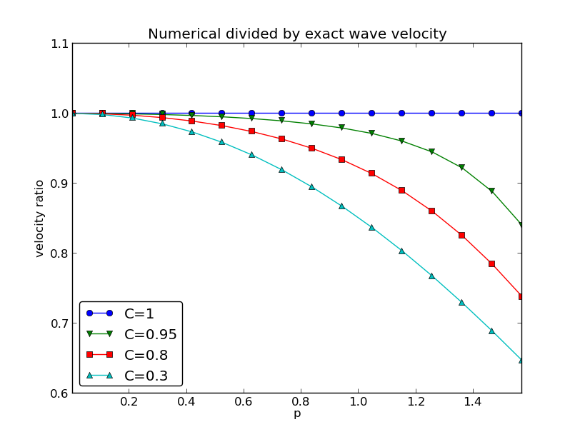
Defining

def r(C, p):
    return 2/(C*p)*asin(C*sin(p))

we can plot \(r(C,p)\) as a function of \(p\) for various values of \(C\), see Figure Figure 2.5. Note that the shortest waves have the most erroneous velocity, and that short waves move more slowly than they should.

We can also easily make a Taylor series expansion in the discretization parameter \(p\):

>>> import sympy as sym
>>> C, p = sym.symbols('C p')
>>> # Compute the 7 first terms around p=0 with no O() term
>>> rs = r(C, p).series(p, 0, 7).removeO()
>>> rs
p**6*(5*C**6/112 - C**4/16 + 13*C**2/720 - 1/5040) +
p**4*(3*C**4/40 - C**2/12 + 1/120) +
p**2*(C**2/6 - 1/6) + 1

>>> # Pick out the leading order term, but drop the constant 1
>>> rs_error_leading_order = (rs - 1).extract_leading_order(p)
>>> rs_error_leading_order
p**2*(C**2/6 - 1/6)

>>> # Turn the series expansion into a Python function
>>> rs_pyfunc = lambdify([C, p], rs, modules='numpy')

>>> # Check: rs_pyfunc is exact (=1) for C=1
>>> rs_pyfunc(1, 0.1)
1.0

Note that without the .removeO() call the series gets an O(x**7) term that makes it impossible to convert the series to a Python function (for, e.g., plotting).

From the rs_error_leading_order expression above, we see that the leading order term in the error of this series expansion is \[ \frac{1}{6}\left(\frac{k\Delta x}{2}\right)^2(C^2-1) = \frac{k^2}{24}\left( c^2\Delta t^2 - \Delta x^2\right), \] pointing to an error \(\Oof{\Delta t^2, \Delta x^2}\), which is compatible with the errors in the difference approximations (\(D_tD_tu\) and \(D_xD_xu\)).

We can do more with a series expansion, e.g., factor it to see how the factor \(C-1\) plays a significant role. To this end, we make a list of the terms, factor each term, and then sum the terms:

>>> rs = r(C, p).series(p, 0, 4).removeO().as_ordered_terms()
>>> rs
[1, C**2*p**2/6 - p**2/6,
 3*C**4*p**4/40 - C**2*p**4/12 + p**4/120,
 5*C**6*p**6/112 - C**4*p**6/16 + 13*C**2*p**6/720 - p**6/5040]
>>> rs = [factor(t) for t in rs]
>>> rs
[1, p**2*(C - 1)*(C + 1)/6,
 p**4*(C - 1)*(C + 1)*(3*C - 1)*(3*C + 1)/120,
 p**6*(C - 1)*(C + 1)*(225*C**4 - 90*C**2 + 1)/5040]
>>> rs = sum(rs)  # Python's sum function sums the list
>>> rs
p**6*(C - 1)*(C + 1)*(225*C**4 - 90*C**2 + 1)/5040 +
p**4*(C - 1)*(C + 1)*(3*C - 1)*(3*C + 1)/120 +
p**2*(C - 1)*(C + 1)/6 + 1

We see from the last expression that \(C=1\) makes all the terms in rs vanish. Since we already know that the numerical solution is exact for \(C=1\), the remaining terms in the Taylor series expansion will also contain factors of \(C-1\) and cancel for \(C=1\).

2.44 Extending the analysis to 2D and 3D

The typical analytical solution of a 2D wave equation \[ u_{tt} = c^2(u_{xx} + u_{yy}), \] is a wave traveling in the direction of \(\kk = k_x\ii + k_y\jj\), where \(\ii\) and \(\jj\) are unit vectors in the \(x\) and \(y\) directions, respectively (\(\ii\) should not be confused with \(i=\sqrt{-1}\) here). Such a wave can be expressed by \[ u(x,y,t) = g(k_xx + k_yy - kct) \] for some twice differentiable function \(g\), or with \(\omega =kc\), \(k=|\kk|\): \[ u(x,y,t) = g(k_xx + k_yy - \omega t)\tp \] We can, in particular, build a solution by adding complex Fourier components of the form \[ e^{(i(k_xx + k_yy - \omega t))} \tp \] A discrete 2D wave equation can be written as \[ \lbrack D_tD_t u = c^2(D_xD_x u + D_yD_y u)\rbrack^n_{q,r} \tp \tag{2.61}\] This equation admits a Fourier component \[ u^n_{q,r} = e^{\left( i(k_x q\Delta x + k_y r\Delta y - \tilde\omega n\Delta t)\right)}, \tag{2.62}\] as solution. Letting the operators \(D_tD_t\), \(D_xD_x\), and \(D_yD_y\) act on \(u^n_{q,r}\) from (2.62) transforms (2.61) to \[ \frac{4}{\Delta t^2}\sin^2\left(\frac{\tilde\omega\Delta t}{2}\right) = c^2 \frac{4}{\Delta x^2}\sin^2\left(\frac{k_x\Delta x}{2}\right) + c^2 \frac{4}{\Delta y^2}\sin^2\left(\frac{k_y\Delta y}{2}\right) \tp \] or \[ \sin^2\left(\frac{\tilde\omega\Delta t}{2}\right) = C_x^2\sin^2 p_x + C_y^2\sin^2 p_y, \] where we have eliminated the factor 4 and introduced the symbols \[ C_x = \frac{c\Delta t}{\Delta x},\quad C_y = \frac{c\Delta t}{\Delta y}, \quad p_x = \frac{k_x\Delta x}{2},\quad p_y = \frac{k_y\Delta y}{2}\tp \] For a real-valued \(\tilde\omega\) the right-hand side must be less than or equal to unity in absolute value, requiring in general that \[ C_x^2 + C_y^2 \leq 1 \tp \tag{2.63}\] This gives the stability criterion, more commonly expressed directly in an inequality for the time step: \[ \Delta t \leq \frac{1}{c} \left( \frac{1}{\Delta x^2} + \frac{1}{\Delta y^2}\right)^{-\halfi} \tag{2.64}\] A similar, straightforward analysis for the 3D case leads to \[ \Delta t \leq \frac{1}{c}\left( \frac{1}{\Delta x^2} + \frac{1}{\Delta y^2} + \frac{1}{\Delta z^2}\right)^{-\halfi} \] In the case of a variable coefficient \(c^2=c^2(\xpoint)\), we must use the worst-case value \[ \bar c = \sqrt{\max_{\xpoint\in\Omega} c^2(\xpoint)} \] in the stability criteria. Often, especially in the variable wave velocity case, it is wise to introduce a safety factor \(\beta\in (0,1]\) too: \[ \Delta t \leq \beta \frac{1}{\bar c} \left( \frac{1}{\Delta x^2} + \frac{1}{\Delta y^2} + \frac{1}{\Delta z^2}\right)^{-\halfi} \] The exact numerical dispersion relations in 2D and 3D becomes, for constant \(c\),

\[\begin{align} \tilde\omega &= \frac{2}{\Delta t}\sin^{-1}\left( \left( C_x^2\sin^2 p_x + C_y^2\sin^2 p_y\right)^\half\right),\\ \tilde\omega &= \frac{2}{\Delta t}\sin^{-1}\left( \left( C_x^2\sin^2 p_x + C_y^2\sin^2 p_y + C_z^2\sin^2 p_z\right)^\half\right)\tp \end{align}\]

We can visualize the numerical dispersion error in 2D much like we did in 1D. To this end, we need to reduce the number of parameters in \(\tilde\omega\). The direction of the wave is parameterized by the polar angle \(\theta\), which means that \[ k_x = k\sin\theta,\quad k_y=k\cos\theta\tp \] A simplification is to set \(\Delta x=\Delta y=h\). Then \(C_x=C_y=c\Delta t/h\), which we call \(C\). Also, \[ p_x=\half kh\cos\theta,\quad p_y=\half kh\sin\theta\tp \] The numerical frequency \(\tilde\omega\) is now a function of three parameters:

• \(C\), reflecting the number of cells a wave is displaced during a time step,
• \(p=\half kh\), reflecting the number of cells per wave length in space,
• \(\theta\), expressing the direction of the wave.

We want to visualize the error in the numerical frequency. To avoid having \(\Delta t\) as a free parameter in \(\tilde\omega\), we work with \(\tilde c/c = \tilde\omega/(kc)\). The coefficient in front of the \(\sin^{-1}\) factor is then \[ \frac{2}{kc\Delta t} = \frac{2}{2kc\Delta t h/h} = \frac{1}{Ckh} = \frac{2}{Cp}, \] and \[ \frac{\tilde c}{c} = \frac{2}{Cp} \sin^{-1}\left(C\left(\sin^2 (p\cos\theta) + \sin^2(p\sin\theta) \right)^\half\right)\tp \] We want to visualize this quantity as a function of \(p\) and \(\theta\) for some values of \(C\leq 1\). It is instructive to make color contour plots of \(1-\tilde c/c\) in polar coordinates with \(\theta\) as the angular coordinate and \(p\) as the radial coordinate.

The stability criterion (2.63) becomes \(C\leq C_{\max} = 1/\sqrt{2}\) in the present 2D case with the \(C\) defined above. Let us plot \(1-\tilde c/c\) in polar coordinates for \(C_{\max}, 0.9C_{\max}, 0.5C_{\max}, 0.2C_{\max}\). The program below does the somewhat tricky work in Matplotlib, and the result appears in Figure Figure 2.6. From the figure we clearly see that the maximum \(C\) value gives the best results, and that waves whose propagation direction makes an angle of 45 degrees with an axis are the most accurate.

Figure 2.6: Error in numerical dispersion in 2D.

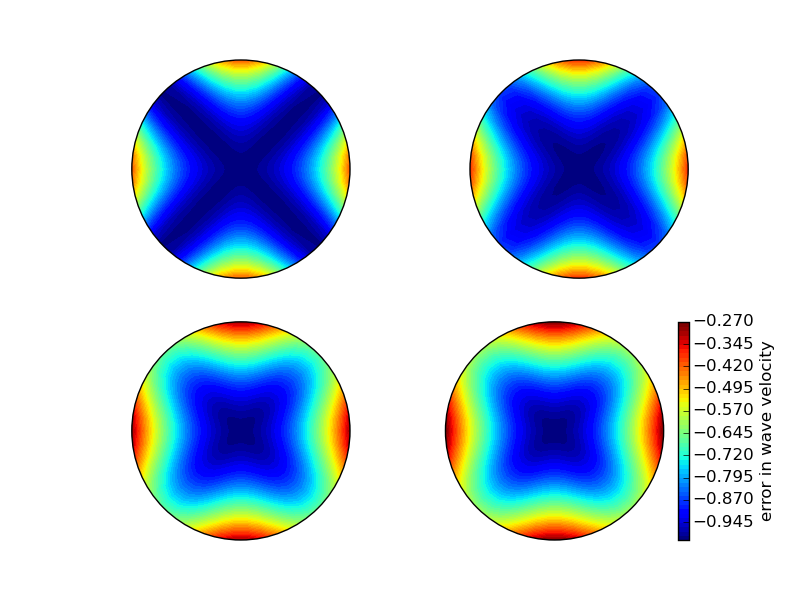
2.45 Multi-dimensional wave equations

A natural next step is to consider extensions of the methods for various variants of the one-dimensional wave equation to two-dimensional (2D) and three-dimensional (3D) versions of the wave equation.

2.46 Multi-dimensional wave equations

The general wave equation in \(d\) space dimensions, with constant wave velocity \(c\), can be written in the compact form \[ \frac{\partial^2 u}{\partial t^2} = c^2\nabla^2 u\text{ for }\xpoint\in\Omega\subset\Real^d,\ t\in (0,T] , \tag{2.65}\] where \[ \nabla^2 u = \frac{\partial^2 u}{\partial x^2} + \frac{\partial^2 u}{\partial y^2} , \] in a 2D problem (\(d=2\)) and \[ \nabla^2 u = \frac{\partial^2 u}{\partial x^2} + \frac{\partial^2 u}{\partial y^2} + \frac{\partial^2 u}{\partial z^2}, \] in three space dimensions (\(d=3\)).

Many applications involve variable coefficients, and the general wave equation in \(d\) dimensions is in this case written as \[ \varrho\frac{\partial^2 u}{\partial t^2} = \nabla\cdot (q\nabla u) + f\text{ for }\xpoint\in\Omega\subset\Real^d,\ t\in (0,T], \tag{2.66}\] which in, e.g., 2D becomes \[ \varrho(x,y) \frac{\partial^2 u}{\partial t^2} = \frac{\partial}{\partial x}\left( q(x,y) \frac{\partial u}{\partial x}\right) + \frac{\partial}{\partial y}\left( q(x,y) \frac{\partial u}{\partial y}\right) + f(x,y,t) \tp \] To save some writing and space we may use the index notation, where subscript \(t\), \(x\), or \(y\) means differentiation with respect to that coordinate. For example,

\[\begin{align*} \frac{\partial^2 u}{\partial t^2} &= u_{tt},\\ \frac{\partial}{\partial y}\left( q(x,y) \frac{\partial u}{\partial y}\right) &= (q u_y)_y \end{align*}\] These comments extend straightforwardly to 3D, which means that the 3D versions of the two wave PDEs, with and without variable coefficients, can be stated as

\[ u_{tt} = c^2(u_{xx} + u_{yy} + u_{zz}) + f, \tag{2.67}\] \[ \varrho u_{tt} = (q u_x)_x + (q u_y)_y + (q u_z)_z + f\tp \tag{2.68}\]

At each point of the boundary \(\partial\Omega\) (of \(\Omega\)) we need one boundary condition involving the unknown \(u\). The boundary conditions are of three principal types:

1. \(u\) is prescribed (\(u=0\) or a known time variation of \(u\) at the boundary points, e.g., modeling an incoming wave),
2. \(\partial u/\partial n = \normalvec\cdot\nabla u\) is prescribed (zero for reflecting boundaries),
3. an open boundary condition (also called radiation condition) is specified to let waves travel undisturbed out of the domain, see Exercise Section 2.36 for details.

All the listed wave equations with second-order derivatives in time need two initial conditions:

1. \(u=I\),
2. \(u_t = V\).

2.47 Mesh

We introduce a mesh in time and in space. The mesh in time consists of time points \[ t_0=0 < t_1 < \cdots < t_{N_t}, \] normally, for wave equation problems, with a constant spacing \(\Delta t= t_{n+1}-t_{n}\), \(n\in\setl{\It}\).

Finite difference methods are easy to implement on simple rectangle- or box-shaped spatial domains. More complicated shapes of the spatial domain require substantially more advanced techniques and implementational efforts (and a finite element method is usually a more convenient approach). On a rectangle- or box-shaped domain, mesh points are introduced separately in the various space directions:

\[\begin{align*} &x_0 < x_1 < \cdots < x_{N_x} \text{ in the }x \text{ direction},\\ &y_0 < y_1 < \cdots < y_{N_y} \text{ in the }y \text{ direction},\\ &z_0 < z_1 < \cdots < z_{N_z} \text{ in the }z \text{ direction}\tp \end{align*}\] We can write a general mesh point as \((x_i,y_j,z_k,t_n)\), with \(i\in\Ix\), \(j\in\Iy\), \(k\in\Iz\), and \(n\in\It\).

It is a very common choice to use constant mesh spacings: \(\Delta x = x_{i+1}-x_{i}\), \(i\in\setl{\Ix}\), \(\Delta y = y_{j+1}-y_{j}\), \(j\in\setl{\Iy}\), and \(\Delta z = z_{k+1}-z_{k}\), \(k\in\setl{\Iz}\). With equal mesh spacings one often introduces \(h = \Delta x = \Delta y =\Delta z\).

The unknown \(u\) at mesh point \((x_i,y_j,z_k,t_n)\) is denoted by \(u^{n}_{i,j,k}\). In 2D problems we just skip the \(z\) coordinate (by assuming no variation in that direction: \(\partial/\partial z=0\)) and write \(u^n_{i,j}\).

2.48 Discretization

Two- and three-dimensional wave equations are easily discretized by assembling building blocks for discretization of 1D wave equations, because the multi-dimensional versions just contain terms of the same type as those in 1D.

2.48.1 Discretizing the PDEs

Equation (2.67) can be discretized as \[ [D_tD_t u = c^2(D_xD_x u + D_yD_yu + D_zD_z u) + f]^n_{i,j,k} \tp \] A 2D version might be instructive to write out in detail: \[ [D_tD_t u = c^2(D_xD_x u + D_yD_yu) + f]^n_{i,j}, \] which becomes \[ \frac{u^{n+1}_{i,j} - 2u^{n}_{i,j} + u^{n-1}_{i,j}}{\Delta t^2} = c^2 \frac{u^{n}_{i+1,j} - 2u^{n}_{i,j} + u^{n}_{i-1,j}}{\Delta x^2} + c^2 \frac{u^{n}_{i,j+1} - 2u^{n}_{i,j} + u^{n}_{i,j-1}}{\Delta y^2} + f^n_{i,j}, \] Assuming, as usual, that all values at time levels \(n\) and \(n-1\) are known, we can solve for the only unknown \(u^{n+1}_{i,j}\). The result can be compactly written as \[ u^{n+1}_{i,j} = 2u^n_{i,j} + u^{n-1}_{i,j} + c^2\Delta t^2[D_xD_x u + D_yD_y u]^n_{i,j}\tp \tag{2.69}\]

As in the 1D case, we need to develop a special formula for \(u^1_{i,j}\) where we combine the general scheme for \(u^{n+1}_{i,j}\), when \(n=0\), with the discretization of the initial condition: \[ [D_{2t}u = V]^0_{i,j}\quad\Rightarrow\quad u^{-1}_{i,j} = u^1_{i,j} - 2\Delta t V_{i,j} \tp \] The result becomes, in compact form, \[ u^{1}_{i,j} = u^0_{i,j} -2\Delta V_{i,j} + {\half} c^2\Delta t^2[D_xD_x u + D_yD_y u]^0_{i,j}\tp \tag{2.70}\]

The PDE (2.68) with variable coefficients is discretized term by term using the corresponding elements from the 1D case: \[ [\varrho D_tD_t u = (D_x\overline{q}^x D_x u + D_y\overline{q}^y D_yu + D_z\overline{q}^z D_z u) + f]^n_{i,j,k} \tp \] When written out and solved for the unknown \(u^{n+1}_{i,j,k}\), one gets the scheme

\[\begin{align*} u^{n+1}_{i,j,k} &= - u^{n-1}_{i,j,k} + 2u^{n}_{i,j,k} + \\ &\quad \frac{1}{\varrho_{i,j,k}}\frac{1}{\Delta x^2} ( \half(q_{i,j,k} + q_{i+1,j,k})(u^{n}_{i+1,j,k} - u^{n}_{i,j,k}) - \\ &\qquad\qquad \half(q_{i-1,j,k} + q_{i,j,k})(u^{n}_{i,j,k} - u^{n}_{i-1,j,k})) + \\ &\quad \frac{1}{\varrho_{i,j,k}}\frac{1}{\Delta y^2} ( \half(q_{i,j,k} + q_{i,j+1,k})(u^{n}_{i,j+1,k} - u^{n}_{i,j,k}) - \\ &\qquad\qquad\half(q_{i,j-1,k} + q_{i,j,k})(u^{n}_{i,j,k} - u^{n}_{i,j-1,k})) + \\ &\quad \frac{1}{\varrho_{i,j,k}}\frac{1}{\Delta z^2} ( \half(q_{i,j,k} + q_{i,j,k+1})(u^{n}_{i,j,k+1} - u^{n}_{i,j,k}) -\\ &\qquad\qquad \half(q_{i,j,k-1} + q_{i,j,k})(u^{n}_{i,j,k} - u^{n}_{i,j,k-1})) + \\ &\quad \Delta t^2 f^n_{i,j,k} \end{align*}\]

Also here we need to develop a special formula for \(u^1_{i,j,k}\) by combining the scheme for \(n=0\) with the discrete initial condition, which is just a matter of inserting \(u^{-1}_{i,j,k}=u^1_{i,j,k} - 2\Delta tV_{i,j,k}\) in the scheme and solving for \(u^1_{i,j,k}\).

2.48.2 Handling boundary conditions where \(u\) is known

The schemes listed above are valid for the internal points in the mesh. After updating these, we need to visit all the mesh points at the boundaries and set the prescribed \(u\) value.

2.48.3 Discretizing the Neumann condition

The condition \(\partial u/\partial n = 0\) was implemented in 1D by discretizing it with a \(D_{2x}u\) centered difference, followed by eliminating the fictitious \(u\) point outside the mesh by using the general scheme at the boundary point. Alternatively, one can introduce ghost cells and update a ghost value for use in the Neumann condition. Exactly the same ideas are reused in multiple dimensions.

Consider the condition \(\partial u/\partial n = 0\) at a boundary \(y=0\) of a rectangular domain \([0, L_x]\times [0,L_y]\) in 2D. The normal direction is then in \(-y\) direction, so \[ \frac{\partial u}{\partial n} = -\frac{\partial u}{\partial y}, \] and we set \[ [-D_{2y} u = 0]^n_{i,0}\quad\Rightarrow\quad \frac{u^n_{i,1}-u^n_{i,-1}}{2\Delta y} = 0 \tp \] From this it follows that \(u^n_{i,-1}=u^n_{i,1}\). The discretized PDE at the boundary point \((i,0)\) reads \[ \frac{u^{n+1}_{i,0} - 2u^{n}_{i,0} + u^{n-1}_{i,0}}{\Delta t^2} = c^2 \frac{u^{n}_{i+1,0} - 2u^{n}_{i,0} + u^{n}_{i-1,0}}{\Delta x^2} + c^2 \frac{u^{n}_{i,1} - 2u^{n}_{i,0} + u^{n}_{i,-1}}{\Delta y^2} + f^n_{i,j}, \] We can then just insert \(u^n_{i,1}\) for \(u^n_{i,-1}\) in this equation and solve for the boundary value \(u^{n+1}_{i,0}\), just as was done in 1D.

From these calculations, we see a pattern: the general scheme applies at the boundary \(j=0\) too if we just replace \(j-1\) by \(j+1\). Such a pattern is particularly useful for implementations. The details follow from the explained 1D case in Section Section 2.17.

The alternative approach to eliminating fictitious values outside the mesh is to have \(u^n_{i,-1}\) available as a ghost value. The mesh is extended with one extra line (2D) or plane (3D) of ghost cells at a Neumann boundary. In the present example it means that we need a line with ghost cells below the \(y\) axis. The ghost values must be updated according to \(u^{n+1}_{i,-1}=u^{n+1}_{i,1}\).

2.49 The 2D Wave Equation with Devito

Extending the wave solver to two dimensions illustrates the power of Devito’s dimension-agnostic approach. The same symbolic patterns apply, and Devito automatically generates optimized 2D stencils.

2.49.1 The 2D Wave Equation

The two-dimensional wave equation on \([0, L_x] \times [0, L_y]\) is: \[ \frac{\partial^2 u}{\partial t^2} = c^2 \left( \frac{\partial^2 u}{\partial x^2} + \frac{\partial^2 u}{\partial y^2} \right) = c^2 \nabla^2 u \tag{2.71}\]

where \(\nabla^2 u = u_{xx} + u_{yy}\) is the Laplacian.

2.49.2 Devito’s Dimension-Agnostic Laplacian

Devito provides the .laplace attribute that works in any dimension:

from devito import Grid, TimeFunction

# 2D grid
grid = Grid(shape=(Nx + 1, Ny + 1), extent=(Lx, Ly))

# 2D wave field
u = TimeFunction(name='u', grid=grid, time_order=2, space_order=2)

# The Laplacian works the same as in 1D!
laplacian = u.laplace  # Returns u_xx + u_yy automatically

This is one of Devito’s key strengths: the same code pattern scales from 1D to 2D to 3D without changes.

2.49.3 CFL Stability Condition in 2D

The stability condition in 2D is more restrictive than in 1D: \[ C = c \cdot \Delta t \cdot \sqrt{\frac{1}{\Delta x^2} + \frac{1}{\Delta y^2}} \le 1 \]

For equal grid spacing \(\Delta x = \Delta y = h\): \[ \Delta t \le \frac{h}{c\sqrt{2}} \]

Compared to the 1D condition \(\Delta t \le h/c\), the 2D condition allows smaller time steps by a factor of \(1/\sqrt{2} \approx 0.707\).

2.49.4 The 2D Solver

The src.wave module provides solve_wave_2d:

from src.wave import solve_wave_2d
import numpy as np

# Initial condition: 2D standing wave
def I(X, Y):
    return np.sin(np.pi * X) * np.sin(np.pi * Y)

result = solve_wave_2d(
    Lx=1.0, Ly=1.0,    # Domain size
    c=1.0,              # Wave speed
    Nx=50, Ny=50,       # Grid points
    T=1.0,              # Final time
    C=0.5,              # Courant number
    I=I,                # Initial displacement
)

# Result is a 2D array
print(result.u.shape)  # (51, 51)

2.49.5 2D Boundary Conditions

Dirichlet conditions must be applied on all four boundaries:

from devito import Eq

t_dim = grid.stepping_dim
x_dim, y_dim = grid.dimensions

# Boundary conditions (u = 0 on all boundaries)
bc_x0 = Eq(u[t_dim + 1, 0, y_dim], 0)      # Left
bc_xN = Eq(u[t_dim + 1, Nx, y_dim], 0)     # Right
bc_y0 = Eq(u[t_dim + 1, x_dim, 0], 0)      # Bottom
bc_yN = Eq(u[t_dim + 1, x_dim, Ny], 0)     # Top

2.49.6 Standing Waves in 2D

The exact solution for the initial condition \(I(x, y) = \sin(\pi x/L_x) \sin(\pi y/L_y)\) with \(V = 0\) is: \[ u(x, y, t) = \sin\left(\frac{\pi x}{L_x}\right) \sin\left(\frac{\pi y}{L_y}\right) \cos(\omega t) \]

where the angular frequency is: \[ \omega = c \pi \sqrt{\frac{1}{L_x^2} + \frac{1}{L_y^2}} \]

This can be used for verification:

from src.wave import convergence_test_wave_2d

grid_sizes, errors, rate = convergence_test_wave_2d(
    grid_sizes=[10, 20, 40, 80],
    T=0.25,
    C=0.5,
)

print(f"Observed convergence rate: {rate:.2f}")  # Should be ~2.0

2.49.7 Visualizing 2D Solutions

For 2D problems, surface plots and contour plots are useful:

import matplotlib.pyplot as plt
from mpl_toolkits.mplot3d import Axes3D

result = solve_wave_2d(Lx=1.0, Ly=1.0, Nx=50, Ny=50, T=0.5, C=0.5)

X, Y = np.meshgrid(result.x, result.y, indexing='ij')

fig = plt.figure(figsize=(12, 5))

# Surface plot
ax1 = fig.add_subplot(121, projection='3d')
ax1.plot_surface(X, Y, result.u, cmap='viridis')
ax1.set_xlabel('x')
ax1.set_ylabel('y')
ax1.set_zlabel('u')
ax1.set_title(f't = {result.t:.3f}')

# Contour plot
ax2 = fig.add_subplot(122)
c = ax2.contourf(X, Y, result.u, levels=20, cmap='RdBu_r')
plt.colorbar(c, ax=ax2)
ax2.set_xlabel('x')
ax2.set_ylabel('y')
ax2.set_title('Contour plot')
ax2.set_aspect('equal')

2.49.8 Animation of 2D Waves

from matplotlib.animation import FuncAnimation

result = solve_wave_2d(
    Lx=1.0, Ly=1.0, Nx=50, Ny=50, T=2.0, C=0.5,
    save_history=True,
)

fig, ax = plt.subplots()
X, Y = np.meshgrid(result.x, result.y, indexing='ij')

vmax = np.abs(result.u_history).max()
im = ax.contourf(X, Y, result.u_history[0], levels=20,
                 cmap='RdBu_r', vmin=-vmax, vmax=vmax)

def update(frame):
    ax.clear()
    ax.contourf(X, Y, result.u_history[frame], levels=20,
                cmap='RdBu_r', vmin=-vmax, vmax=vmax)
    ax.set_title(f't = {result.t_history[frame]:.3f}')
    ax.set_aspect('equal')
    return []

anim = FuncAnimation(fig, update, frames=len(result.t_history),
                     interval=50)

2.49.9 From 2D to 3D

The pattern extends naturally to three dimensions. In Devito, the main changes are:

1. Add a third dimension to the grid
2. The .laplace attribute automatically includes \(u_{zz}\)

# 3D grid
grid = Grid(shape=(Nx+1, Ny+1, Nz+1), extent=(Lx, Ly, Lz))

# 3D wave field
u = TimeFunction(name='u', grid=grid, time_order=2, space_order=2)

# The PDE is unchanged!
pde = u.dt2 - c**2 * u.laplace

The CFL condition in 3D becomes: \[ \Delta t \le \frac{h}{c\sqrt{3}} \]

for equal grid spacing in all directions.

2.49.10 Computational Considerations

2D and 3D wave simulations can become computationally expensive. Devito helps through:

• Automatic parallelization: Set OMP_NUM_THREADS for OpenMP
• Cache optimization: Loop tiling is applied automatically
• GPU support: Use platform='nvidiaX' for CUDA execution

For large-scale simulations, the generated C code is highly optimized and can match hand-tuned implementations.

2.49.11 Summary

Key points for 2D wave equations with Devito:

1. The .laplace attribute handles the dimension automatically
2. CFL conditions are more restrictive (factor of \(1/\sqrt{d}\) in \(d\) dimensions)
3. Boundary conditions must be applied on all boundaries
4. Visualization requires surface/contour plots and animations
5. The same code patterns extend to 3D with minimal changes

Devito’s abstraction means we write the physics once and let the framework handle the computational complexity across dimensions.

2.50 Absorbing Boundary Conditions

When we simulate wave propagation in unbounded or semi-infinite domains, we must truncate the computational domain to a finite region. The artificial boundaries introduced by this truncation cause spurious reflections that contaminate the solution. Absorbing boundary conditions (ABCs) are techniques designed to minimize these reflections, allowing outgoing waves to leave the domain as if the boundary were not there.

This section surveys the main ABC approaches, compares their effectiveness, and provides Devito (Louboutin et al. 2019) implementations for each. The treatment applies to the scalar acoustic wave equation \[ \frac{\partial^2 u}{\partial t^2} = c^2 \nabla^2 u, \tag{2.72}\] but the ideas extend to elastic waves and electromagnetics (see Section 8.5.4 for the electromagnetic case).

2.50.1 The Problem of Artificial Boundaries

Consider a point source radiating in an infinite 2D domain. The exact solution consists of an outward-propagating circular wavefront that never returns. If we truncate the domain to a rectangle and impose Dirichlet conditions \(u = 0\) on all boundaries, the outgoing wave reflects back into the interior as if it hit a rigid wall.

The ideal boundary condition is the Sommerfeld radiation condition: \[ \lim_{r \to \infty} \sqrt{r} \left( \frac{\partial u}{\partial r} - \frac{1}{c}\frac{\partial u}{\partial t} \right) = 0, \tag{2.73}\] which states that at large distances from the source, the solution behaves as an outgoing wave. This is a condition at infinity — it cannot be directly applied at a finite boundary.

All practical ABCs are approximations of the Sommerfeld condition (Engquist and Majda 1977). The key metric for evaluating them is the reflection coefficient \(R\): the ratio of reflected to incident wave amplitude. An ideal ABC has \(R = 0\); Dirichlet boundaries have \(R = 1\) (total reflection with sign change).

2.50.2 First-Order Absorbing BC

The simplest ABC is the first-order radiation condition (Clayton and Engquist 1977): \[ \frac{\partial u}{\partial t} + c \frac{\partial u}{\partial n} = 0 \quad \text{on } \Gamma, \tag{2.74}\] where \(\partial/\partial n\) is the outward normal derivative on the boundary \(\Gamma\). This condition is exact for plane waves at normal incidence: substituting \(u = f(x - ct)\) into (2.74) gives \(-cf' + cf' = 0\).

Discretization. At the right boundary \(x = L_x\) (grid point \(i = N_x\)), we use forward difference in time and backward difference in space: \[ \frac{u_{N_x}^{n+1} - u_{N_x}^n}{\Delta t} + c \frac{u_{N_x}^n - u_{N_x-1}^n}{\Delta x} = 0, \] giving the explicit update: \[ u_{N_x}^{n+1} = u_{N_x}^n - \frac{c \Delta t}{\Delta x} \left( u_{N_x}^n - u_{N_x-1}^n \right). \tag{2.75}\]

Similar formulas apply to the other three boundaries (left, top, bottom), with appropriate sign changes for the normal direction.

Limitations in 2D. The first-order ABC is exact only for waves arriving at normal incidence (\(\theta = 0\)). For a plane wave arriving at angle \(\theta\) to the normal, the reflection coefficient is: \[ R(\theta) \approx \frac{1 - \cos\theta}{1 + \cos\theta}. \] At \(\theta = 45°\), this gives \(R \approx 0.17\) (17% reflection), and as \(\theta \to 90°\) (grazing incidence), \(R \to 1\). For a point source producing waves at all angles, the first-order ABC provides only moderate improvement over Dirichlet boundaries.

Devito implementation. The first-order ABC on all four boundaries of a 2D domain:

from devito import Grid, TimeFunction, Eq, Operator, Constant, solve

grid = Grid(shape=(Nx+1, Ny+1), extent=(Lx, Ly))
u = TimeFunction(name='u', grid=grid, time_order=2, space_order=2)
c_sq = Constant(name='c_sq')
c_val = Constant(name='c_val')

# Interior PDE
pde = u.dt2 - c_sq * u.laplace
stencil = Eq(u.forward, solve(pde, u.forward),
             subdomain=grid.interior)

# First-order ABC on each boundary
t = grid.stepping_dim
x_dim, y_dim = grid.dimensions
dx_s, dy_s = grid.spacing

# Right boundary: u_t + c*u_x = 0
bc_right = Eq(u[t+1, Nx, y_dim],
    u[t, Nx, y_dim]
    - c_val * dt / dx_s * (u[t, Nx, y_dim] - u[t, Nx-1, y_dim]))

# Left boundary: u_t - c*u_x = 0
bc_left = Eq(u[t+1, 0, y_dim],
    u[t, 0, y_dim]
    + c_val * dt / dx_s * (u[t, 1, y_dim] - u[t, 0, y_dim]))

# Similar for top and bottom...

Corner treatment. In 2D, corner grid points belong to two boundaries simultaneously (e.g., the point \((0, 0)\) lies on both the left and bottom boundaries). The equations above update corners twice — once for each boundary — with the last-applied equation overwriting the first. For first-order ABCs this double-update is acceptable because both boundary operators produce similar values at corners. Higher-order methods such as HABC (Section 2.50.6) require explicit corner treatment to maintain accuracy and stability.

2.50.3 Damping Layers (Sponge Zones)

Instead of modifying the boundary condition, damping layers (also called sponge zones) add a dissipative term to the PDE in a region near the boundary (Cerjan et al. 1985; Sochacki et al. 1987). The modified equation is: \[ \frac{\partial^2 u}{\partial t^2} + \gamma(\mathbf{x}) \frac{\partial u}{\partial t} = c^2 \nabla^2 u, \tag{2.76}\] where \(\gamma(\mathbf{x})\) is a damping coefficient that is zero in the interior domain and ramps up smoothly in the absorbing layer: \[ \gamma(d) = \sigma_{\max} \left(\frac{d}{W}\right)^p, \quad 0 \le d \le W, \tag{2.77}\] with \(d\) being the distance into the absorbing layer, \(W\) the layer width, \(p\) the polynomial order (typically 2–3), and \(\sigma_{\max}\) the maximum damping value.

The damping term \(\gamma u_t\) removes energy from the wave as it propagates through the sponge layer. The key design parameters are:

• Layer width \(W\): Wider layers absorb more but increase computational cost. Typical values are 10–40 grid cells.
• Maximum damping \(\sigma_{\max}\): Too large causes reflections at the layer interface; too small allows waves to pass through. A good starting value is \(\sigma_{\max} \approx 3c/W\).
• Polynomial order \(p\): Higher order gives a smoother transition. \(p = 3\) is a common choice.

Devito implementation. The damping layer is straightforward to implement using a Function for the damping profile:

Snippet (tested)

This code is included from src/book_snippets/damping_layer_2d_wave.py and exercised by pytest (see tests/test_book_snippets.py).

import numpy as np
from devito import Constant, Eq, Function, Grid, Operator, TimeFunction, solve

# 2D wave equation with sponge (damping) layer absorbing boundaries.
Lx, Ly = 2.0, 2.0
Nx, Ny = 80, 80
c = 1.0
CFL = 0.5
pad = 15  # damping layer width in grid cells

dx, dy = Lx / Nx, Ly / Ny
dt = CFL / (c * np.sqrt(1 / dx**2 + 1 / dy**2))
Nt = int(round(1.0 / dt))
dt = 1.0 / Nt

grid = Grid(shape=(Nx + 1, Ny + 1), extent=(Lx, Ly))
u = TimeFunction(name="u", grid=grid, time_order=2, space_order=2)

# Gaussian initial condition at center
x = np.linspace(0, Lx, Nx + 1)
y = np.linspace(0, Ly, Ny + 1)
X, Y = np.meshgrid(x, y, indexing="ij")
u.data[0, :, :] = np.exp(-((X - 1.0) ** 2 + (Y - 1.0) ** 2) / (2 * 0.1**2))
u.data[1, :, :] = u.data[0, :, :]

# Build polynomial damping profile: zero in interior, ramps near edges
# sigma_max chosen from theory: 3*c / W where W = pad*dx
sigma_max = 3.0 * c / (pad * dx)
damp = Function(name="damp", grid=grid)
gamma = np.zeros((Nx + 1, Ny + 1))
for i in range(pad):
    d = (pad - i) / pad
    gamma[i, :] = np.maximum(gamma[i, :], sigma_max * d**3)
    gamma[Nx - i, :] = np.maximum(gamma[Nx - i, :], sigma_max * d**3)
for j in range(pad):
    d = (pad - j) / pad
    gamma[:, j] = np.maximum(gamma[:, j], sigma_max * d**3)
    gamma[:, Ny - j] = np.maximum(gamma[:, Ny - j], sigma_max * d**3)
damp.data[:] = gamma

# PDE with damping: u_tt + damp*u_t = c^2 * laplace(u)
c_sq = Constant(name="c_sq")
pde = u.dt2 + damp * u.dt - c_sq * u.laplace
stencil = Eq(u.forward, solve(pde, u.forward))

t_dim = grid.stepping_dim
x_dim, y_dim = grid.dimensions
bc = [
    Eq(u[t_dim + 1, 0, y_dim], 0),
    Eq(u[t_dim + 1, Nx, y_dim], 0),
    Eq(u[t_dim + 1, x_dim, 0], 0),
    Eq(u[t_dim + 1, x_dim, Ny], 0),
]
op = Operator([stencil] + bc)

for _n in range(2, Nt + 1):
    op.apply(time_m=1, time_M=1, dt=dt, c_sq=c**2)
    u.data[0, :, :] = u.data[1, :, :]
    u.data[1, :, :] = u.data[2, :, :]

RESULT = float(np.max(np.abs(u.data[1, pad:-pad, pad:-pad])))

The damping profile is zero in the interior and increases toward the boundary following (2.77). The solve function in Devito automatically handles the modified PDE, producing the correct time-stepping stencil including the damping term.

Effectiveness. With a 20-cell layer and \(p = 3\), damping layers typically achieve 90–95% reflection reduction compared to Dirichlet boundaries (Dolci et al. 2022). The main advantage is simplicity: the method requires only adding one term to the PDE and defining the damping profile. The main disadvantage is the relatively wide layer needed for good absorption.

2.50.4 Perfectly Matched Layer (PML)

The Perfectly Matched Layer (PML), introduced by Berenger (Berenger 1994), achieves superior absorption through complex coordinate stretching. The fundamental idea is to replace the real coordinate \(x\) with a complex-valued stretched coordinate: \[ \tilde{x} = x + \frac{1}{j\omega} \int_0^x \sigma_x(x')\, dx', \tag{2.78}\] where \(\sigma_x(x')\) is a conductivity profile and \(\omega\) is the angular frequency. This transformation makes plane waves decay exponentially in the PML region while ensuring zero reflection at the PML interface for any angle of incidence and any frequency.

Auxiliary-field formulation. For implementation, the complex coordinate stretching leads to a modified PDE with auxiliary fields. For the 2D acoustic wave equation, the PML-modified system is: \[\begin{align} \frac{\partial^2 u}{\partial t^2} + (\sigma_x + \sigma_y) \frac{\partial u}{\partial t} + \sigma_x \sigma_y\, u &= c^2 \nabla^2 u + \frac{\partial p_x}{\partial t} + \frac{\partial p_y}{\partial t}, \label{eq:pml-main} \\ \frac{\partial p_x}{\partial t} &= -\sigma_x p_x + (\sigma_y - \sigma_x)\, c^2 \frac{\partial^2 u}{\partial x^2}, \label{eq:pml-px} \\ \frac{\partial p_y}{\partial t} &= -\sigma_y p_y + (\sigma_x - \sigma_y)\, c^2 \frac{\partial^2 u}{\partial y^2}, \label{eq:pml-py} \end{align}\] where \(p_x\) and \(p_y\) are auxiliary fields that are nonzero only in the PML region, and \(\sigma_x(x)\), \(\sigma_y(y)\) are conductivity profiles following (2.77). In the interior where \(\sigma_x = \sigma_y = 0\), the system reduces to the standard wave equation.

Devito implementation. The PML is implemented using the Grote-Sim formulation with separate directional damping profiles \(\sigma_x(x)\) and \(\sigma_y(y)\), plus auxiliary TimeFunction fields phi_x and phi_y. The maximum damping is chosen from PML theory to achieve a target reflection coefficient \(R\): \[ \sigma_{\max} = \frac{(p+1)\, c\, \ln(1/R)}{2W}, \tag{2.79}\] where \(p\) is the polynomial order and \(W\) is the layer width.

Snippet (tested)

This code is included from src/book_snippets/pml_wave_2d.py and exercised by pytest (see tests/test_book_snippets.py).

import numpy as np
from devito import Constant, Eq, Function, Grid, Operator, TimeFunction, solve

# 2D wave equation with split-field PML absorbing boundaries.
# Uses separate directional damping (sigma_x, sigma_y) and auxiliary
# fields (phi_x, phi_y) following the Grote-Sim formulation.
Lx, Ly = 2.0, 2.0
Nx, Ny = 80, 80
c = 1.0
CFL = 0.5
pad = 15  # PML width in grid cells

dx, dy = Lx / Nx, Ly / Ny
dt = CFL / (c * np.sqrt(1 / dx**2 + 1 / dy**2))
Nt = int(round(1.0 / dt))
dt = 1.0 / Nt

grid = Grid(shape=(Nx + 1, Ny + 1), extent=(Lx, Ly))
u = TimeFunction(name="u", grid=grid, time_order=2, space_order=2)

# Gaussian initial condition at center
x = np.linspace(0, Lx, Nx + 1)
y = np.linspace(0, Ly, Ny + 1)
X, Y = np.meshgrid(x, y, indexing="ij")
u.data[0, :, :] = np.exp(-((X - 1.0) ** 2 + (Y - 1.0) ** 2) / (2 * 0.1**2))
u.data[1, :, :] = u.data[0, :, :]

# Build directional PML damping profiles
# sigma_max from PML theory: (p+1)*c*ln(1/R)/(2*W)
R_target = 1e-3
order = 3
W = pad * dx
sigma_max = (order + 1) * c * np.log(1.0 / R_target) / (2 * W)

sigma_x_arr = np.zeros((Nx + 1, Ny + 1))
sigma_y_arr = np.zeros((Nx + 1, Ny + 1))
for i in range(pad):
    d = (pad - i) / pad
    sigma_x_arr[i, :] = sigma_max * d**order
    sigma_x_arr[Nx - i, :] = sigma_max * d**order
for j in range(pad):
    d = (pad - j) / pad
    sigma_y_arr[:, j] = sigma_max * d**order
    sigma_y_arr[:, Ny - j] = sigma_max * d**order

sigma_x_fn = Function(name="sigma_x", grid=grid)
sigma_y_fn = Function(name="sigma_y", grid=grid)
sigma_x_fn.data[:] = sigma_x_arr
sigma_y_fn.data[:] = sigma_y_arr

# Auxiliary fields for the split-field PML
phi_x = TimeFunction(name="phi_x", grid=grid, time_order=1, space_order=2)
phi_y = TimeFunction(name="phi_y", grid=grid, time_order=1, space_order=2)

# Grote-Sim PML equation:
# u_tt + (sigma_x + sigma_y)*u_t + sigma_x*sigma_y*u
#   = c^2*laplace(u) + d(phi_x)/dx + d(phi_y)/dy
c_sq = Constant(name="c_sq")
pde = (u.dt2
       + (sigma_x_fn + sigma_y_fn) * u.dt
       + sigma_x_fn * sigma_y_fn * u
       - c_sq * u.laplace
       - phi_x.dx - phi_y.dy)
stencil_u = Eq(u.forward, solve(pde, u.forward))

# Auxiliary field updates (forward Euler):
# phi_x_t = -sigma_x*phi_x + c^2*(sigma_y - sigma_x)*u_x
# phi_y_t = -sigma_y*phi_y + c^2*(sigma_x - sigma_y)*u_y
dt_sym = grid.stepping_dim.spacing
eq_phi_x = Eq(phi_x.forward,
              phi_x + dt_sym * (
                  -sigma_x_fn * phi_x
                  + c_sq * (sigma_y_fn - sigma_x_fn) * u.dx))
eq_phi_y = Eq(phi_y.forward,
              phi_y + dt_sym * (
                  -sigma_y_fn * phi_y
                  + c_sq * (sigma_x_fn - sigma_y_fn) * u.dy))

t_dim = grid.stepping_dim
x_dim, y_dim = grid.dimensions
bc = [
    Eq(u[t_dim + 1, 0, y_dim], 0),
    Eq(u[t_dim + 1, Nx, y_dim], 0),
    Eq(u[t_dim + 1, x_dim, 0], 0),
    Eq(u[t_dim + 1, x_dim, Ny], 0),
]
op = Operator([stencil_u, eq_phi_x, eq_phi_y] + bc)

for _n in range(2, Nt + 1):
    op.apply(time_m=1, time_M=1, dt=dt, c_sq=c**2)
    u.data[0, :, :] = u.data[1, :, :]
    u.data[1, :, :] = u.data[2, :, :]
    phi_x.data[1, :, :] = phi_x.data[0, :, :]
    phi_y.data[1, :, :] = phi_y.data[0, :, :]

RESULT = float(np.max(np.abs(u.data[1, pad:-pad, pad:-pad])))

The auxiliary fields vanish in the interior (where \(\sigma_x = \sigma_y = 0\)) and are updated with forward Euler in the PML region. The key advantage of the split-field approach is that each direction is damped independently, providing angle-independent absorption.

Effectiveness. With optimally chosen parameters per (2.79), the PML achieves approximately 95% reflection reduction with a layer of only 10–15 cells (Dolci et al. 2022), making it more efficient per grid cell than simple damping layers with heuristic parameters.

The Convolutional PML (CPML) variant (Roden and Gedney 2000) offers improved stability for certain media types by using a recursive convolution formulation. The efficient wave-equation PML of Grote and Sim (2010) provides further optimizations for acoustic applications.

2.50.5 Second-Order Higdon ABC

Higher-order ABCs improve on the first-order condition by absorbing waves at multiple angles simultaneously. Higdon (Higdon 1986, 1987) proposed a product formula: \[ \prod_{j=1}^{P} \left( \frac{\partial}{\partial t} - c_j \frac{\partial}{\partial n} \right) u = 0 \quad \text{on } \Gamma, \tag{2.80}\] where \(c_j = c / \cos\theta_j\) and \(\theta_j\) are chosen angles of incidence. The order-\(P\) Higdon condition exactly absorbs plane waves arriving at any of the \(P\) specified angles.

Derivation for \(P = 2\). With angles \(\theta_1 = 0°\) and \(\theta_2 = 45°\), the product of two first-order operators gives: \[ \left(\frac{\partial}{\partial t} + c \frac{\partial}{\partial n}\right) \left(\frac{\partial}{\partial t} + \frac{c}{\cos 45°} \frac{\partial}{\partial n}\right) u = 0. \] Expanding and discretizing with the averaging parameters \(a = b = 0.5\) (centered in time and space), this yields a nine-point stencil involving \(u\) at three time levels (\(n-1, n, n+1\)) and three spatial points (boundary, +1, +2 interior). Solving for the boundary value \(u_0^{n+1}\) gives an explicit update formula.

The stencil coefficients for each first-order factor are: \[\begin{align} g_{j1} &= \cos\theta_j \cdot (1-a)/\Delta t, \quad g_{j2} = \cos\theta_j \cdot a/\Delta t, \label{eq:higdon-g12}\\ g_{j3} &= \cos\theta_j \cdot (1-b) \cdot c/\Delta h, \quad g_{j4} = \cos\theta_j \cdot b \cdot c/\Delta h, \label{eq:higdon-g34} \end{align}\] where \(\Delta h\) is the grid spacing normal to the boundary. These combine into four coefficients per factor: \(c_{j1} = g_{j1} + g_{j3}\), \(c_{j2} = -g_{j1} + g_{j4}\), \(c_{j3} = g_{j2} - g_{j3}\), \(c_{j4} = -g_{j2} - g_{j4}\).

The boundary value is then: \[ u_0^{n+1} = \frac{1}{c_{11} c_{21}} \sum_{k} \alpha_k \cdot u_k, \] where the sum runs over the eight remaining stencil contributions from the product \(c_{1\cdot} \otimes c_{2\cdot}\).

Devito implementation. The Higdon ABC is applied as a post-processing step after the interior wave equation update. The Devito operator solves the standard wave equation with Dirichlet placeholder BCs, then the Higdon stencil overwrites boundary values:

Snippet (tested)

This code is included from src/book_snippets/higdon_abc_2d_wave.py and exercised by pytest (see tests/test_book_snippets.py).

import numpy as np
from devito import Constant, Eq, Grid, Operator, TimeFunction, solve

# 2D wave equation with second-order Higdon ABC (P=2, angles 0 and pi/4).
# Absorbs waves at normal and 45-degree incidence exactly.
Lx, Ly = 2.0, 2.0
Nx, Ny = 80, 80
c = 1.0
CFL = 0.5

dx, dy = Lx / Nx, Ly / Ny
dt = CFL / (c * np.sqrt(1 / dx**2 + 1 / dy**2))
Nt = int(round(1.0 / dt))
dt = 1.0 / Nt

grid = Grid(shape=(Nx + 1, Ny + 1), extent=(Lx, Ly))
u = TimeFunction(name="u", grid=grid, time_order=2, space_order=2)

# Gaussian initial condition at center
x = np.linspace(0, Lx, Nx + 1)
y = np.linspace(0, Ly, Ny + 1)
X, Y = np.meshgrid(x, y, indexing="ij")
u.data[0, :, :] = np.exp(-((X - 1.0) ** 2 + (Y - 1.0) ** 2) / (2 * 0.1**2))
u.data[1, :, :] = u.data[0, :, :]

# Interior wave equation (Dirichlet BCs as placeholder)
c_sq = Constant(name="c_sq")
pde = u.dt2 - c_sq * u.laplace
stencil = Eq(u.forward, solve(pde, u.forward), subdomain=grid.interior)

t_dim = grid.stepping_dim
x_dim, y_dim = grid.dimensions
bc = [
    Eq(u[t_dim + 1, 0, y_dim], 0),
    Eq(u[t_dim + 1, Nx, y_dim], 0),
    Eq(u[t_dim + 1, x_dim, 0], 0),
    Eq(u[t_dim + 1, x_dim, Ny], 0),
]
op = Operator([stencil] + bc)

# Higdon P=2 coefficients (angles 0 and pi/4, a=b=0.5)
from src.wave.abc_methods import _apply_higdon_bc

for _n in range(2, Nt + 1):
    op.apply(time_m=1, time_M=1, dt=dt, c_sq=c**2)
    # Apply Higdon ABC at all four boundaries
    _apply_higdon_bc(u.data, Nx, Ny, c, dt, dx, dy)
    u.data[0, :, :] = u.data[1, :, :]
    u.data[1, :, :] = u.data[2, :, :]

RESULT = float(np.max(np.abs(u.data[1, 5:-5, 5:-5])))

2.50.6 Hybrid Absorbing Boundary Conditions (HABC)

The most effective strategy combines a Higdon ABC at the boundary with a thin weighted absorption layer just inside the boundary (Dolci et al. 2022; Liu and Sen 2018). The HABC uses a non-linear weight function \(w(k)\) that blends the Higdon correction with the wave equation solution: \[ u_k^{n+1} = (1 - w_k)\, u_k^{\text{wave}} + w_k\, u_k^{\text{Higdon}}, \tag{2.81}\] where \(k\) is the distance from the boundary in grid cells, \(u^{\text{wave}}\) is the standard wave equation update, and \(u^{\text{Higdon}}\) is the Higdon boundary value extrapolated into the layer.

The weight function has three regions:

1. Flat region (\(k \le P\)): \(w_k = 1\) — the Higdon correction is applied in full strength at and near the boundary.
2. Decay region (\(P < k < W\)): \(w_k = \left(\frac{W - k}{W - P}\right)^\alpha\) — polynomial decay toward the interior.
3. Interior (\(k = W\)): \(w_k = 0\) — no correction applied.

The exponent \(\alpha = 1 + 0.15(W - P)\) controls how quickly the correction fades. This non-linear blending smooths the transition from the ABC to the interior, avoiding the artificial interface reflections that plague simple damping layers.

Corner treatment. At corners where x- and y-layer corrections overlap, the HABC takes the more absorptive value (minimum absolute value) to avoid over-correction artifacts.

Devito implementation. Like the Higdon ABC, the HABC is applied as a post-processing step. The key difference is that the correction extends into the absorption layer with decreasing weight:

Snippet (tested)

This code is included from src/book_snippets/habc_wave_2d.py and exercised by pytest (see tests/test_book_snippets.py).

import numpy as np
from devito import Constant, Eq, Grid, Operator, TimeFunction, solve

# 2D wave equation with Hybrid Absorbing Boundary Condition (HABC).
# Combines second-order Higdon ABC with a weighted absorption layer
# for near-optimal reflection reduction with minimal layer width.
Lx, Ly = 2.0, 2.0
Nx, Ny = 80, 80
c = 1.0
CFL = 0.5
pad = 10  # HABC layer width (much thinner than damping)

dx, dy = Lx / Nx, Ly / Ny
dt = CFL / (c * np.sqrt(1 / dx**2 + 1 / dy**2))
Nt = int(round(1.0 / dt))
dt = 1.0 / Nt

grid = Grid(shape=(Nx + 1, Ny + 1), extent=(Lx, Ly))
u = TimeFunction(name="u", grid=grid, time_order=2, space_order=2)

# Gaussian initial condition at center
x = np.linspace(0, Lx, Nx + 1)
y = np.linspace(0, Ly, Ny + 1)
X, Y = np.meshgrid(x, y, indexing="ij")
u.data[0, :, :] = np.exp(-((X - 1.0) ** 2 + (Y - 1.0) ** 2) / (2 * 0.1**2))
u.data[1, :, :] = u.data[0, :, :]

# Interior wave equation with Dirichlet BCs (overwritten by HABC)
c_sq = Constant(name="c_sq")
pde = u.dt2 - c_sq * u.laplace
stencil = Eq(u.forward, solve(pde, u.forward), subdomain=grid.interior)

t_dim = grid.stepping_dim
x_dim, y_dim = grid.dimensions
bc = [
    Eq(u[t_dim + 1, 0, y_dim], 0),
    Eq(u[t_dim + 1, Nx, y_dim], 0),
    Eq(u[t_dim + 1, x_dim, 0], 0),
    Eq(u[t_dim + 1, x_dim, Ny], 0),
]
op = Operator([stencil] + bc)

# HABC weights and Higdon correction
from src.wave.abc_methods import _apply_habc_correction, create_habc_weights

weights = create_habc_weights(pad)

for _n in range(2, Nt + 1):
    op.apply(time_m=1, time_M=1, dt=dt, c_sq=c**2)
    _apply_habc_correction(u.data, Nx, Ny, c, dt, dx, dy, pad, weights)
    u.data[0, :, :] = u.data[1, :, :]
    u.data[1, :, :] = u.data[2, :, :]

RESULT = float(np.max(np.abs(u.data[1, pad:-pad, pad:-pad])))

Dolci et al. (2022) show that the HABC achieves up to 99% reflection reduction with only 5–10 cells of absorbing layer — significantly more cost-effective than simple damping layers that require 20–40 cells for comparable performance.

2.50.7 Comparison and Practical Recommendations

The following table summarizes the ABC methods covered in this section. Performance numbers are representative for a 2D point-source test problem with constant velocity (Dolci et al. 2022; Liu and Sen 2018).

Table 2.1: Comparison of absorbing boundary conditions for the 2D wave equation.

Method	Layer width	Reflection reduction	Extra memory	Complexity
Dirichlet	0	0% (baseline)	None	Trivial
First-order ABC	0	~50–70%	None	Simple
Damping layer	20–40 cells	~90–95%	\(\gamma\) profile	Simple
PML (split-field)	10–15 cells	~95%	\(\phi_x, \phi_y\) fields	Moderate
Higdon \(P{=}2\)	0	~80–90%	None	Moderate
HABC (Higdon + weights)	5–10 cells	~99%	Weight array	Complex

Practical recommendations:

1. For pedagogical use and prototyping: Start with the first-order ABC. It is easy to implement and provides a noticeable improvement over Dirichlet boundaries.

2. For general-purpose simulation: Use a damping layer with 20 cells and cubic polynomial ramp (\(p = 3\)). This provides good absorption with minimal implementation effort.

3. For production-quality results: Use PML with 10–15 cells. The extra implementation complexity pays off in smaller computational domains for the same accuracy.

4. For research and large-scale applications: Consider the hybrid HABC-Higdon approach. The 2–5 cell layer thickness can significantly reduce computational cost in 3D simulations where the absorbing region is a substantial fraction of the domain.

5. Always verify: Compare your ABC solution against a reference computed on a larger domain to ensure reflections are acceptably small. The measure_reflection function in src.wave.abc_methods automates this comparison.

2.50.8 Exercises

Exercise 1: First-order ABC in 2D. Implement the first-order absorbing boundary condition (2.75) on all four boundaries of a 2D domain using Devito. Use a Gaussian point source at the center and run the simulation long enough for the wavefront to reach all boundaries. Compare the solution to one with Dirichlet boundaries by plotting snapshots at the same time. Measure the reflection coefficient using the energy in the interior after the wavefront has passed.

Exercise 2: Damping layer parameter study. Using the damping layer implementation from Section 2.50.3, investigate the effect of:

1. Layer width: \(W = 5, 10, 20, 40\) cells
2. Polynomial order: \(p = 1, 2, 3, 4\)
3. Maximum damping: \(\sigma_{\max} = 10, 50, 100, 500\)

For each parameter, measure the reflection coefficient and plot the results. Which parameter has the strongest effect? What is the minimum layer width that achieves less than 5% reflection?

Exercise 3: PML vs. damping comparison. Implement both the PML (Section 2.50.4) and damping layer (Section 2.50.3) methods on the same test problem. For a fair comparison, use the same total layer width (e.g., 15 cells) for both methods. Compare:

1. The reflection coefficient
2. The total computational time
3. The memory usage (number of grid functions)

Discuss when the PML’s superior per-cell absorption justifies its additional complexity.

Exercise 4 (Advanced): Second-order Higdon ABC. Implement a second-order Higdon ABC (2.80) with \(P = 2\) using angles \(\theta_1 = 0°\) and \(\theta_2 = 60°\). The discrete form at the right boundary requires expanding the product of two first-order operators: \[ \left(\frac{\partial}{\partial t} + c \frac{\partial}{\partial x}\right) \left(\frac{\partial}{\partial t} + \frac{c}{\cos 60°} \frac{\partial}{\partial x}\right) u = 0. \]

Discretize this using centered differences and solve for \(u_{N_x}^{n+1}\). Compare the reflection at various angles against the first-order ABC. How much improvement do you observe at \(\theta = 45°\) and \(\theta = 60°\)?

2.51 Applications of wave equations

This section presents a range of wave equation models for different physical phenomena. Although many wave motion problems in physics can be modeled by the standard linear wave equation, or a similar formulation with a system of first-order equations, there are some exceptions. Perhaps the most important is water waves: these are modeled by the Laplace equation with time-dependent boundary conditions at the water surface (long water waves, however, can be approximated by a standard wave equation, see Section Section 2.58). Quantum mechanical waves constitute another example where the waves are governed by the Schrödinger equation, i.e., not by a standard wave equation. Many wave phenomena also need to take nonlinear effects into account when the wave amplitude is significant. Shock waves in the air is a primary example.

The derivations in the following are very brief. Those with a firm background in continuum mechanics will probably have enough knowledge to fill in the details, while other readers will hopefully get some impression of the physics and approximations involved when establishing wave equation models.

2.52 Waves on a string

Figure 2.7: Discrete string model with point masses connected by elastic strings.

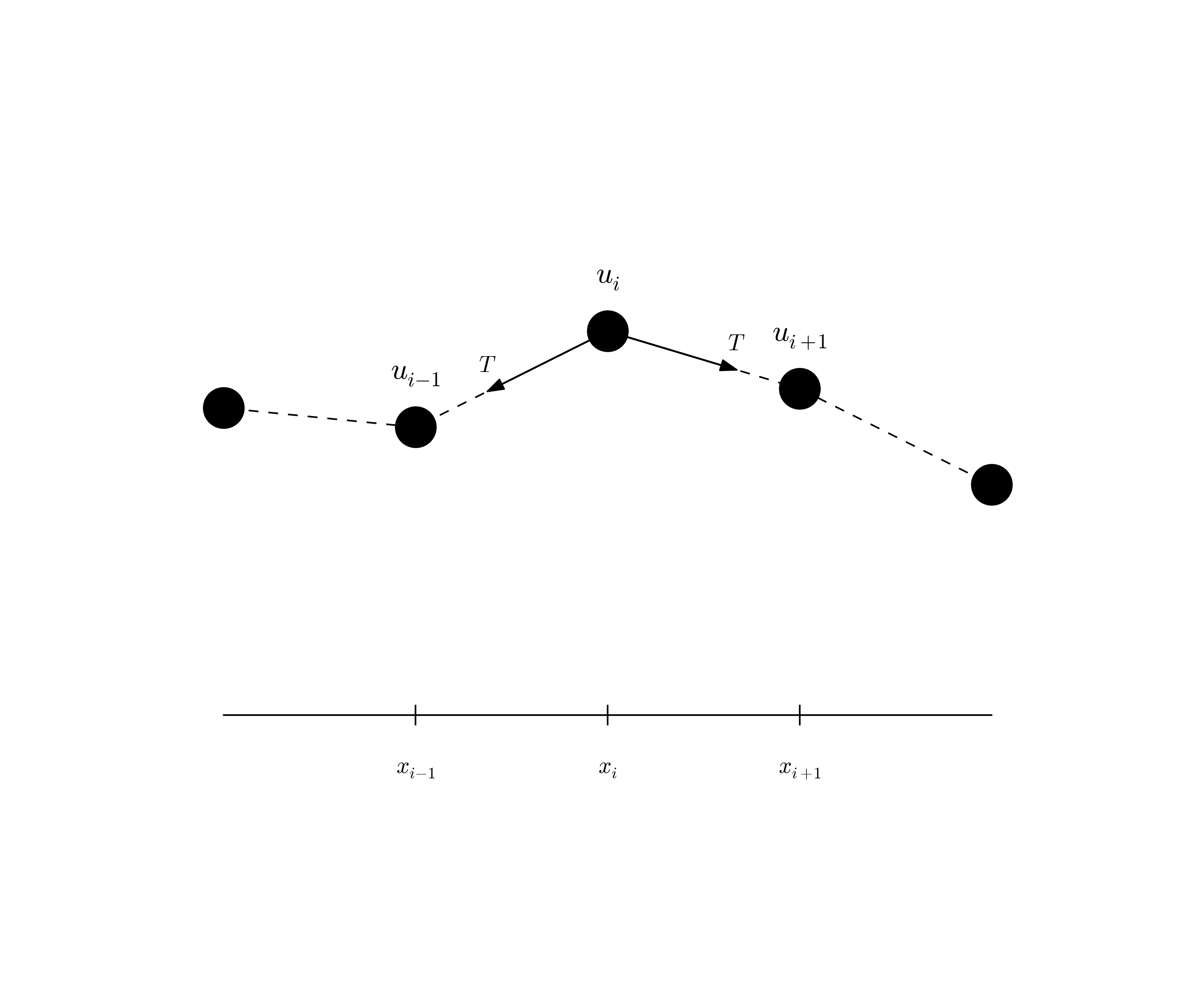
Figure Figure 2.7 shows a model we may use to derive the equation for waves on a string. The string is modeled as a set of discrete point masses (at mesh points) with elastic strings in between. The string has a large constant tension \(T\). We let the mass at mesh point \(x_i\) be \(m_i\). The displacement of this mass point in the \(y\) direction is denoted by \(u_i(t)\).

The motion of mass \(m_i\) is governed by Newton’s second law of motion. The position of the mass at time \(t\) is \(x_i\ii + u_i(t)\jj\), where \(\ii\) and \(\jj\) are unit vectors in the \(x\) and \(y\) direction, respectively. The acceleration is then \(u_i''(t)\jj\). Two forces are acting on the mass as indicated in Figure Figure 2.7. The force \(\T^{-}\) acting toward the point \(x_{i-1}\) can be decomposed as \[ \T^{-} = -T\sin\phi\ii -T\cos\phi\jj, \] where \(\phi\) is the angle between the force and the line \(x=x_i\). Let \(\Delta u_i = u_i - u_{i-1}\) and let \(\Delta s_i = \sqrt{\Delta u_i^2 + (x_i - x_{i-1})^2}\) be the distance from mass \(m_{i-1}\) to mass \(m_i\). It is seen that \(\cos\phi = \Delta u_i/\Delta s_i\) and \(\sin\phi = (x_{i}-x_{i-1})/\Delta s\) or \(\Delta x/\Delta s_i\) if we introduce a constant mesh spacing \(\Delta x = x_i - x_{i-1}\). The force can then be written \[ \T^{-} = -T\frac{\Delta x}{\Delta s_i}\ii - T\frac{\Delta u_i}{\Delta s_i}\jj \tp \] The force \(\T^{+}\) acting toward \(x_{i+1}\) can be calculated in a similar way: \[ \T^{+} = T\frac{\Delta x}{\Delta s_{i+1}}\ii + T\frac{\Delta u_{i+1}}{\Delta s_{i+1}}\jj \tp \] Newton’s second law becomes \[ m_iu_i''(t)\jj = \T^{+} + \T^{-}, \] which gives the component equations

\[ T\frac{\Delta x}{\Delta s_i} = T\frac{\Delta x}{\Delta s_{i+1}}, \tag{2.82}\] \[ m_iu_i''(t) = T\frac{\Delta u_{i+1}}{\Delta s_{i+1}} - T\frac{\Delta u_i}{\Delta s_i}\tp \tag{2.83}\]

A basic reasonable assumption for a string is small displacements \(u_i\) and small displacement gradients \(\Delta u_i/\Delta x\). For small \(g=\Delta u_i/\Delta x\) we have that \[ \Delta s_i = \sqrt{\Delta u_i^2 + \Delta x^2} = \Delta x\sqrt{1 + g^2} + \Delta x (1 + {\half}g^2 + \mathcal{O}(g^4)) \approx \Delta x \tp \] Equation (2.82) is then simply the identity \(T=T\), while (2.83) can be written as \[ m_iu_i''(t) = T\frac{\Delta u_{i+1}}{\Delta x} - T\frac{\Delta u_i}{\Delta x}, \] which upon division by \(\Delta x\) and introducing the density \(\varrho_i = m_i/\Delta x\) becomes \[ \varrho_i u_i''(t) = T\frac{1}{\Delta x^2} \left( u_{i+1} - 2u_i + u_{i-1}\right) \tp \tag{2.84}\] We can now choose to approximate \(u_i''\) by a finite difference in time and get the discretized wave equation, \[ \varrho_i \frac{1}{\Delta t^2} \left(u^{n+1}_i - 2u^n_i - u^{n-1}_i\right) = T\frac{1}{\Delta x^2} \left( u_{i+1} - 2u_i + u_{i-1}\right)\tp \] On the other hand, we may go to the continuum limit \(\Delta x\rightarrow 0\) and replace \(u_i(t)\) by \(u(x,t)\), \(\varrho_i\) by \(\varrho(x)\), and recognize that the right-hand side of (2.84) approaches \(\partial^2 u/\partial x^2\) as \(\Delta x\rightarrow 0\). We end up with the continuous model for waves on a string: \[ \varrho\frac{\partial^2 u}{\partial t^2} = T\frac{\partial^2 u}{\partial x^2} \tp \tag{2.85}\] Note that the density \(\varrho\) may change along the string, while the tension \(T\) is a constant. With variable wave velocity \(c(x) = \sqrt{T/\varrho(x)}\) we can write the wave equation in the more standard form \[ \frac{\partial^2 u}{\partial t^2} = c^2(x)\frac{\partial^2 u}{\partial x^2} \tp \tag{2.86}\] Because of the way \(\varrho\) enters the equations, the variable wave velocity does not appear inside the derivatives as in many other versions of the wave equation. However, most strings of interest have constant \(\varrho\).

The end points of a string are fixed so that the displacement \(u\) is zero. The boundary conditions are therefore \(u=0\).

2.52.1 Damping

Air resistance and non-elastic effects in the string will contribute to reduce the amplitudes of the waves so that the motion dies out after some time. This damping effect can be modeled by a term \(bu_t\) on the left-hand side of the equation \[ \varrho\frac{\partial^2 u}{\partial t^2} + b\frac{\partial u}{\partial t} = T\frac{\partial^2 u}{\partial x^2} \tp \tag{2.87}\] The parameter \(b\geq 0\) is small for most wave phenomena, but the damping effect may become significant in long time simulations.

2.52.2 External forcing

It is easy to include an external force acting on the string. Say we have a vertical force \(\tilde f_i\jj\) acting on mass \(m_i\), modeling the effect of gravity on a string. This force affects the vertical component of Newton’s law and gives rise to an extra term \(\tilde f(x,t)\) on the right-hand side of (2.85). In the model (2.86) we would add a term \(f(x,t) = \tilde f(x,t)/\varrho(x)\).

2.52.3 Modeling the tension via springs

We assumed, in the derivation above, that the tension in the string, \(T\), was constant. It is easy to check this assumption by modeling the string segments between the masses as standard springs, where the force (tension \(T\)) is proportional to the elongation of the spring segment. Let \(k\) be the spring constant, and set \(T_i=k\Delta \ell\) for the tension in the spring segment between \(x_{i-1}\) and \(x_i\), where \(\Delta\ell\) is the elongation of this segment from the tension-free state. A basic feature of a string is that it has high tension in the equilibrium position \(u=0\). Let the string segment have an elongation \(\Delta\ell_0\) in the equilibrium position. After deformation of the string, the elongation is \(\Delta \ell = \Delta \ell_0 + \Delta s_i\): \(T_i = k(\Delta \ell_0 + \Delta s_i)\approx k(\Delta \ell_0 + \Delta x)\). This shows that \(T_i\) is independent of \(i\). Moreover, the extra approximate elongation \(\Delta x\) is very small compared to \(\Delta\ell_0\), so we may well set \(T_i = T = k\Delta\ell_0\). This means that the tension is completely dominated by the initial tension determined by the tuning of the string. The additional deformations of the spring during the vibrations do not introduce significant changes in the tension.

2.53 Elastic waves in a rod

Consider an elastic rod subject to a hammer impact at the end. This experiment will give rise to an elastic deformation pulse that travels through the rod. A mathematical model for longitudinal waves along an elastic rod starts with the general equation for deformations and stresses in an elastic medium, \[ \varrho\uu_{tt} = \nabla\cdot\stress + \varrho\f, \tag{2.88}\] where \(\varrho\) is the density, \(\uu\) the displacement field, \(\stress\) the stress tensor, and \(\f\) body forces. The latter has normally no impact on elastic waves.

For stationary deformation of an elastic rod, aligned with the \(x\) axis, one has that \(\sigma_{xx} = Eu_x\), with all other stress components being zero. The parameter \(E\) is known as Young’s modulus. Moreover, we set \(\uu = u(x,t)\ii\) and neglect the radial contraction and expansion (where Poisson’s ratio is the important parameter). Assuming that this simple stress and deformation field is a good approximation, (2.88) simplifies to \[ \varrho\frac{\partial^2 u}{\partial t^2} = \frac{\partial}{\partial x} \left( E\frac{\partial u}{\partial x}\right) \tp \tag{2.89}\]

The associated boundary conditions are \(u\) or \(\sigma_{xx}=Eu_x\) known, typically \(u=0\) for a fixed end and \(\sigma_{xx}=0\) for a free end.

2.54 Waves on a membrane

Think of a thin, elastic membrane with shape as a circle or rectangle. This membrane can be brought into oscillatory motion and will develop elastic waves. We can model this phenomenon somewhat similar to waves in a rod: waves in a membrane are simply the two-dimensional counterpart. We assume that the material is deformed in the \(z\) direction only and write the elastic displacement field on the form \(\uu (x,y,t) = w(x,y,t)\ii\). The \(z\) coordinate is omitted since the membrane is thin and all properties are taken as constant throughout the thickness. Inserting this displacement field in Newton’s 2nd law of motion (2.88) results in \[ \varrho\frac{\partial^2 w}{\partial t^2} = \frac{\partial}{\partial x} \left( \mu\frac{\partial w}{\partial x}\right) + \frac{\partial}{\partial y} \left( \mu\frac{\partial w}{\partial y}\right) \tp \tag{2.90}\] This is nothing but a wave equation in \(w(x,y,t)\), which needs the usual initial conditions on \(w\) and \(w_t\) as well as a boundary condition \(w=0\). When computing the stress in the membrane, one needs to split \(\stress\) into a constant high-stress component (since all membranes are normally pre-stressed) plus a component proportional to the displacement and governed by the wave motion.

2.55 The acoustic model for seismic waves

Seismic waves are used to infer properties of subsurface geological structures. The physical model is a heterogeneous elastic medium where sound is propagated by small elastic vibrations. The general mathematical model for deformations in an elastic medium is based on Newton’s second law, \[ \varrho\uu_{tt} = \nabla\cdot\stress + \varrho\f, \tag{2.91}\] and a constitutive law relating \(\stress\) to \(\uu\), often Hooke’s generalized law, \[ \stress = K\nabla\cdot\uu\, \I + G(\nabla\uu + (\nabla\uu)^T - \frac{2}{3}\nabla\cdot\uu\, \I) \tp \tag{2.92}\] Here, \(\uu\) is the displacement field, \(\stress\) is the stress tensor, \(\I\) is the identity tensor, \(\varrho\) is the medium’s density, \(\f\) are body forces (such as gravity), \(K\) is the medium’s bulk modulus and \(G\) is the shear modulus. All these quantities may vary in space, while \(\uu\) and \(\stress\) will also show significant variation in time during wave motion.

The acoustic approximation to elastic waves arises from a basic assumption that the second term in Hooke’s law, representing the deformations that give rise to shear stresses, can be neglected. This assumption can be interpreted as approximating the geological medium by a fluid. Neglecting also the body forces \(\f\), (2.91) becomes \[ \varrho\uu_{tt} = \nabla (K\nabla\cdot\uu ) \tag{2.93}\] Introducing \(p\) as a pressure via \[ p=-K\nabla\cdot\uu, \tag{2.94}\] and dividing (2.93) by \(\varrho\), we get \[ \uu_{tt} = -\frac{1}{\varrho}\nabla p \tp \] Taking the divergence of this equation, using \(\nabla\cdot\uu = -p/K\) from (2.94), gives the acoustic approximation to elastic waves: \[ p_{tt} = K\nabla\cdot\left(\frac{1}{\varrho}\nabla p\right) \tp \tag{2.95}\] This is a standard, linear wave equation with variable coefficients. It is common to add a source term \(s(x,y,z,t)\) to model the generation of sound waves: \[ p_{tt} = K\nabla\cdot\left(\frac{1}{\varrho}\nabla p\right) + s \tp \tag{2.96}\]

A common additional approximation of (2.96) is based on using the chain rule on the right-hand side, \[ K\nabla\cdot\left(\frac{1}{\varrho}\nabla p\right) = \frac{K}{\varrho}\nabla^2 p + K\nabla\left(\frac{1}{\varrho}\right)\cdot \nabla p \approx \frac{K}{\varrho}\nabla^2 p, \] under the assumption that the relative spatial gradient \(\nabla\varrho^{-1} = -\varrho^{-2}\nabla\varrho\) is small. This approximation results in the simplified equation \[ p_{tt} = \frac{K}{\varrho}\nabla^2 p + s \tp \tag{2.97}\]

The acoustic approximations to seismic waves are used for sound waves in the ground, and the Earth’s surface is then a boundary where \(p\) equals the atmospheric pressure \(p_0\) such that the boundary condition becomes \(p=p_0\).

2.55.1 Anisotropy

Quite often in geological materials, the effective wave velocity \(c=\sqrt{K/\varrho}\) is different in different spatial directions because geological layers are compacted, and often twisted, in such a way that the properties in the horizontal and vertical direction differ. With \(z\) as the vertical coordinate, we can introduce a vertical wave velocity \(c_z\) and a horizontal wave velocity \(c_h\), and generalize (2.97) to \[ p_{tt} = c_z^2 p_{zz} + c_h^2 (p_{xx} + p_{yy}) + s \tp \tag{2.98}\]

2.56 Sound waves in liquids and gases

Sound waves arise from pressure and density variations in fluids. The starting point of modeling sound waves is the basic equations for a compressible fluid where we omit viscous (frictional) forces, body forces (gravity, for instance), and temperature effects:

\[ \varrho_t + \nabla\cdot (\varrho \uu) = 0, \tag{2.99}\] \[ \varrho \uu_{t} + \varrho \uu\cdot\nabla\uu = -\nabla p, \tag{2.100}\] \[ \varrho = \varrho (p)\tp \tag{2.101}\] These equations are often referred to as the Euler equations for the motion of a fluid. The parameters involved are the density \(\varrho\), the velocity \(\uu\), and the pressure \(p\). Equation (2.99) reflects mass balance, (2.100) is Newton’s second law for a fluid, with frictional and body forces omitted, and (2.101) is a constitutive law relating density to pressure by thermodynamic considerations. A typical model for (2.101) is the so-called isentropic relation, valid for adiabatic processes where there is no heat transfer: \[ \varrho = \varrho_0\left(\frac{p}{p_0}\right)^{1/\gamma} \tp \tag{2.102}\] Here, \(p_0\) and \(\varrho_0\) are reference values for \(p\) and \(\varrho\) when the fluid is at rest, and \(\gamma\) is the ratio of specific heat at constant pressure and constant volume (\(\gamma = 5/3\) for air).

The key approximation in a mathematical model for sound waves is to assume that these waves are small perturbations to the density, pressure, and velocity. We therefore write

\[\begin{align*} p &= p_0 + \hat p,\\ \varrho &= \varrho_0 + \hat\varrho,\\ \uu &= \hat\uu, \end{align*}\] where we have decomposed the fields in a constant equilibrium value, corresponding to \(\uu=0\), and a small perturbation marked with a hat symbol. By inserting these decompositions in (2.99) and (2.100), neglecting all product terms of small perturbations and/or their derivatives, and dropping the hat symbols, one gets the following linearized PDE system for the small perturbations in density, pressure, and velocity:

\[ \varrho_t + \varrho_0\nabla\cdot\uu = 0, \] \[ \varrho_0\uu_t = -\nabla p\tp \] Now we can eliminate \(\varrho_t\) by differentiating the relation \(\varrho(p)\), \[ \varrho_t = \varrho_0 \frac{1}{\gamma}\left(\frac{p}{p_0}\right)^{1/\gamma-1} \frac{1}{p_0}p_t = \frac{\varrho_0}{\gamma p_0} \left(\frac{p}{p_0}\right)^{1/\gamma-1}p_t \tp \] The product term \(p^{1/\gamma -1}p_t\) can be linearized as \(p_0^{1/\gamma -1}p_t\), resulting in \[ \varrho_t \approx \frac{\varrho_0}{\gamma p_0} p_t \tp \] We then get

\[ p_t + \gamma p_0\nabla\cdot\uu = 0, \tag{2.103}\] \[ \uu_t = -\frac{1}{\varrho_0}\nabla p\tp \tag{2.104}\] Taking the divergence of (2.104) and differentiating (2.103) with respect to time gives the possibility to easily eliminate \(\nabla\cdot\uu_t\) and arrive at a standard, linear wave equation for \(p\): \[ p_{tt} = c^2\nabla^2 p, \] where \(c = \sqrt{\gamma p_0/\varrho_0}\) is the speed of sound in the fluid.

2.57 Spherical waves

Spherically symmetric three-dimensional waves propagate in the radial direction \(r\) only so that \(u = u(r,t)\). The fully three-dimensional wave equation \[ \frac{\partial^2u}{\partial t^2}=\nabla\cdot (c^2\nabla u) + f \] then reduces to the spherically symmetric wave equation \[ \frac{\partial^2u}{\partial t^2}=\frac{1}{r^2}\frac{\partial}{\partial r} \left(c^2(r)r^2\frac{\partial u}{\partial r}\right) + f(r,t),\quad r\in (0,R),\ t>0 \tp \] One can easily show that the function \(v(r,t) = ru(r,t)\) fulfills a standard wave equation in Cartesian coordinates if \(c\) is constant. To this end, insert \(u=v/r\) in \[ \frac{1}{r^2}\frac{\partial}{\partial r} \left(c^2(r)r^2\frac{\partial u}{\partial r}\right) \] to obtain \[ r\left(\frac{d c^2}{dr}\frac{\partial v}{\partial r} + c^2\frac{\partial^2 v}{\partial r^2}\right) - \frac{d c^2}{dr}v \tp \] The two terms in the parenthesis can be combined to \[ r\frac{\partial}{\partial r}\left( c^2\frac{\partial v}{\partial r}\right), \] which is recognized as the variable-coefficient Laplace operator in one Cartesian coordinate. The spherically symmetric wave equation in terms of \(v(r,t)\) now becomes \[ \frac{\partial^2v}{\partial t^2}= \frac{\partial}{\partial r} \left(c^2(r)\frac{\partial v}{\partial r}\right) -\frac{1}{r}\frac{d c^2}{dr}v + rf(r,t),\quad r\in (0,R),\ t>0 \tp \] In the case of constant wave velocity \(c\), this equation reduces to the wave equation in a single Cartesian coordinate called \(r\): \[ \frac{\partial^2v}{\partial t^2}= c^2 \frac{\partial^2 v}{\partial r^2} + rf(r,t),\quad r\in (0,R),\ t>0 \tp \tag{2.105}\] That is, any program for solving the one-dimensional wave equation in a Cartesian coordinate system can be used to solve (2.105), provided the source term is multiplied by the coordinate, and that we divide the Cartesian mesh solution by \(r\) to get the spherically symmetric solution. Moreover, if \(r=0\) is included in the domain, spherical symmetry demands that \(\partial u/\partial r=0\) at \(r=0\), which means that \[ \frac{\partial u}{\partial r} = \frac{1}{r^2}\left( r\frac{\partial v}{\partial r} - v\right) = 0,\quad r=0\tp \] For this to hold in the limit \(r\rightarrow 0\), we must have \(v(0,t)=0\) at least as a necessary condition. In most practical applications, we exclude \(r=0\) from the domain and assume that some boundary condition is assigned at \(r=\epsilon\), for some \(\epsilon >0\).

2.58 The linear shallow water equations

The next example considers water waves whose wavelengths are much larger than the depth and whose wave amplitudes are small. This class of waves may be generated by catastrophic geophysical events, such as earthquakes at the sea bottom, landslides moving into water, or underwater slides (or a combination, as earthquakes frequently release avalanches of masses). For example, a subsea earthquake will normally have an extension of many kilometers but lift the water only a few meters. The wave length will have a size dictated by the earthquake area, which is much lager than the water depth, and compared to this wave length, an amplitude of a few meters is very small. The water is essentially a thin film, and mathematically we can average the problem in the vertical direction and approximate the 3D wave phenomenon by 2D PDEs. Instead of a moving water domain in three space dimensions, we get a horizontal 2D domain with an unknown function for the surface elevation and the water depth as a variable coefficient in the PDEs.

Let \(\eta(x,y,t)\) be the elevation of the water surface, \(H(x,y)\) the water depth corresponding to a flat surface (\(\eta =0\)), \(u(x,y,t)\) and \(v(x,y,t)\) the depth-averaged horizontal velocities of the water. Mass and momentum balance of the water volume give rise to the PDEs involving these quantities:

\[ \eta_t = - (Hu)_x - (Hv)_x \tag{2.106}\] \[ u_t = -g\eta_x, \tag{2.107}\] \[ v_t = -g\eta_y, \tag{2.108}\] where \(g\) is the acceleration of gravity. Equation (2.106) corresponds to mass balance while the other two are derived from momentum balance (Newton’s second law).

The initial conditions associated with (2.106)-(2.108) are \(\eta\), \(u\), and \(v\) prescribed at \(t=0\). A common condition is to have some water elevation \(\eta =I(x,y)\) and assume that the surface is at rest: \(u=v=0\). A subsea earthquake usually means a sufficiently rapid motion of the bottom and the water volume to say that the bottom deformation is mirrored at the water surface as an initial lift \(I(x,y)\) and that \(u=v=0\).

Boundary conditions may be \(\eta\) prescribed for incoming, known waves, or zero normal velocity at reflecting boundaries (steep mountains, for instance): \(un_x + vn_y =0\), where \((n_x,n_y)\) is the outward unit normal to the boundary. More sophisticated boundary conditions are needed when waves run up at the shore, and at open boundaries where we want the waves to leave the computational domain undisturbed.

Equations (2.106), (2.107), and (2.108) can be transformed to a standard, linear wave equation. First, multiply (2.107) and (2.108) by \(H\), differentiate (2.107)) with respect to \(x\) and (2.108) with respect to \(y\). Second, differentiate (2.106) with respect to \(t\) and use that \((Hu)_{xt}=(Hu_t)_x\) and \((Hv)_{yt}=(Hv_t)_y\) when \(H\) is independent of \(t\). Third, eliminate \((Hu_t)_x\) and \((Hv_t)_y\) with the aid of the other two differentiated equations. These manipulations result in a standard, linear wave equation for \(\eta\): \[ \eta_{tt} = (gH\eta_x)_x + (gH\eta_y)_y = \nabla\cdot (gH\nabla\eta) \tp \tag{2.109}\]

In the case we have an initial non-flat water surface at rest, the initial conditions become \(\eta =I(x,y)\) and \(\eta_t=0\). The latter follows from (2.106) if \(u=v=0\), or simply from the fact that the vertical velocity of the surface is \(\eta_t\), which is zero for a surface at rest.

The system (2.106)-(2.108) can be extended to handle a time-varying bottom topography, which is relevant for modeling long waves generated by underwater slides. In such cases the water depth function \(H\) is also a function of \(t\), due to the moving slide, and one must add a time-derivative term \(H_t\) to the left-hand side of (2.106). A moving bottom is best described by introducing \(z=H_0\) as the still-water level, \(z=B(x,y,t)\) as the time- and space-varying bottom topography, so that \(H=H_0-B(x,y,t)\). In the elimination of \(u\) and \(v\) one may assume that the dependence of \(H\) on \(t\) can be neglected in the terms \((Hu)_{xt}\) and \((Hv)_{yt}\). We then end up with a source term in (2.109), because of the moving (accelerating) bottom: \[ \eta_{tt} = \nabla\cdot(gH\nabla\eta) + B_{tt} \tp \tag{2.110}\]

The reduction of (2.110) to 1D, for long waves in a straight channel, or for approximately plane waves in the ocean, is trivial by assuming no change in \(y\) direction (\(\partial/\partial y=0\)): \[ \eta_{tt} = (gH\eta_x)_x + B_{tt} \tp \tag{2.111}\]

2.58.1 Wind drag on the surface

Surface waves are influenced by the drag of the wind, and if the wind velocity some meters above the surface is \((U,V)\), the wind drag gives contributions \(C_V\sqrt{U^2+V^2}U\) and \(C_V\sqrt{U^2+V^2}V\) to (2.107) and (2.108), respectively, on the right-hand sides.

2.58.2 Bottom drag

The waves will experience a drag from the bottom, often roughly modeled by a term similar to the wind drag: \(C_B\sqrt{u^2+v^2}u\) on the right-hand side of (2.107) and \(C_B\sqrt{u^2+v^2}v\) on the right-hand side of (2.108). Note that in this case the PDEs (2.107) and (2.108) become nonlinear and the elimination of \(u\) and \(v\) to arrive at a 2nd-order wave equation for \(\eta\) is not possible anymore.

2.58.3 Effect of the Earth’s rotation

Long geophysical waves will often be affected by the rotation of the Earth because of the Coriolis force. This force gives rise to a term \(fv\) on the right-hand side of (2.107) and \(-fu\) on the right-hand side of (2.108). Also in this case one cannot eliminate \(u\) and \(v\) to work with a single equation for \(\eta\). The Coriolis parameter is \(f=2\Omega\sin\phi\), where \(\Omega\) is the angular velocity of the earth and \(\phi\) is the latitude.

2.59 Waves in blood vessels

The flow of blood in our bodies is basically fluid flow in a network of pipes. Unlike rigid pipes, the walls in the blood vessels are elastic and will increase their diameter when the pressure rises. The elastic forces will then push the wall back and accelerate the fluid. This interaction between the flow of blood and the deformation of the vessel wall results in waves traveling along our blood vessels.

A model for one-dimensional waves along blood vessels can be derived from averaging the fluid flow over the cross section of the blood vessels. Let \(x\) be a coordinate along the blood vessel and assume that all cross sections are circular, though with different radii \(R(x,t)\). The main quantities to compute is the cross section area \(A(x,t)\), the averaged pressure \(P(x,t)\), and the total volume flux \(Q(x,t)\). The area of this cross section is \[ A(x,t) = 2\pi\int_{0}^{R(x,t)} rdr, \] Let \(v_x(x,t)\) be the velocity of blood averaged over the cross section at point \(x\). The volume flux, being the total volume of blood passing a cross section per time unit, becomes \[ Q(x,t) = A(x,t)v_x(x,t) \thinspace \] Mass balance and Newton’s second law lead to the PDEs

\[ \frac{\partial A}{\partial t} + \frac{\partial Q}{\partial x} = 0, \tag{2.112}\] \[ \frac{\partial Q}{\partial t} + \frac{\gamma+2}{\gamma + 1} \frac{\partial}{\partial x}\left(\frac{Q^2}{A}\right) + \frac{A}{\varrho}\frac{\partial P}{\partial x} = -2\pi (\gamma + 2)\frac{\mu}{\varrho}\frac{Q}{A}, \tag{2.113}\] where \(\gamma\) is a parameter related to the velocity profile, \(\varrho\) is the density of blood, and \(\mu\) is the dynamic viscosity of blood.

We have three unknowns \(A\), \(Q\), and \(P\), and two equations (2.112) and (2.113). A third equation is needed to relate the flow to the deformations of the wall. A common form for this equation is \[ \frac{\partial P}{\partial t} + \frac{1}{C} \frac{\partial Q}{\partial x} =0, \tag{2.114}\] where \(C\) is the compliance of the wall, given by the constitutive relation \[ C = \frac{\partial A}{\partial P} + \frac{\partial A}{\partial t}, \] which requires a relationship between \(A\) and \(P\). One common model is to view the vessel wall, locally, as a thin elastic tube subject to an internal pressure. This gives the relation \[ P=P_0 + \frac{\pi h E}{(1-\nu^2)A_0}(\sqrt{A} - \sqrt{A_0}), \] where \(P_0\) and \(A_0\) are corresponding reference values when the wall is not deformed, \(h\) is the thickness of the wall, and \(E\) and \(\nu\) are Young’s modulus and Poisson’s ratio of the elastic material in the wall. The derivative becomes \[ C = \frac{\partial A}{\partial P} = \frac{2(1-\nu^2)A_0}{\pi h E}\sqrt{A_0} + 2\left(\frac{(1-\nu^2)A_0}{\pi h E}\right)^2(P-P_0) \tp \] Another (nonlinear) deformation model of the wall, which has a better fit with experiments, is \[ P = P_0\exp{(\beta (A/A_0 - 1))}, \] where \(\beta\) is some parameter to be estimated. This law leads to \[ C = \frac{\partial A}{\partial P} = \frac{A_0}{\beta P} \tp \] Reduction to the standard wave equation. It is not uncommon to neglect the viscous term on the right-hand side of (2.113) and also the quadratic term with \(Q^2\) on the left-hand side. The reduced equations (2.113) and (2.114) form a first-order linear wave equation system:

\[ C\frac{\partial P}{\partial t} = - \frac{\partial Q}{\partial x}, \] \[ \frac{\partial Q}{\partial t} = - \frac{A}{\varrho}\frac{\partial P}{\partial x}\tp \] These can be combined into standard 1D wave PDE by differentiating the first equation with respect to \(t\) and the second with respect to \(x\), \[ \frac{\partial}{\partial t}\left( C\frac{\partial P}{\partial t} \right) = \frac{\partial}{\partial x}\left( \frac{A}{\varrho}\frac{\partial P}{\partial x}\right), \] which can be approximated by \[ \frac{\partial^2 Q}{\partial t^2} = c^2\frac{\partial^2 Q}{\partial x^2},\quad c = \sqrt{\frac{A}{\varrho C}}, \] where the \(A\) and \(C\) in the expression for \(c\) are taken as constant reference values.

2.60 Electromagnetic waves

Light and radio waves are governed by standard wave equations arising from Maxwell’s general equations. When there are no charges and no currents, as in a vacuum, Maxwell’s equations take the form

\[\begin{align*} \nabla\cdot\pmb{E} &= 0,\\ \nabla\cdot\pmb{B} &= 0,\\ \nabla\times\pmb{E} &= -\frac{\partial\pmb{B}}{\partial t},\\ \nabla\times\pmb{B} &= \mu_0\epsilon_0\frac{\partial\pmb{E}}{\partial t}, \end{align*}\] where \(\epsilon_0=8.854187817620\cdot 10^{-12}\) (F/m) is the permittivity of free space, also known as the electric constant, and \(\mu_0=1.2566370614\cdot 10^{-6}\) (H/m) is the permeability of free space, also known as the magnetic constant. Taking the curl of the two last equations and using the mathematical identity \[ \nabla\times (\nabla\times \pmb{E}) = \nabla(\nabla \cdot \pmb{E}) + \nabla^2\pmb{E} = - \nabla^2\pmb{E}\text{ when }\nabla\cdot\pmb{E}=0, \] gives the wave equation governing the electric and magnetic field: \[\begin{align} \frac{\partial^2\pmb{E}}{\partial t^2} &= c^2\nabla^2\pmb{E},\\ \frac{\partial^2\pmb{B}}{\partial t^2} &= c^2\nabla^2\pmb{B}, \end{align}\] with \(c=1/\sqrt{\mu_0\epsilon_0}\) as the velocity of light. Each component of \(\pmb{E}\) and \(\pmb{B}\) fulfills a wave equation and can hence be solved independently.

2.61 Exercise: Simulate waves on a non-homogeneous string

Simulate waves on a string that consists of two materials with different density. The tension in the string is constant, but the density has a jump at the middle of the string. Experiment with different sizes of the jump and produce animations that visualize the effect of the jump on the wave motion.

According to Section Section 2.52,

the density enters the mathematical model as \(\varrho\) in \(\varrho u_{tt} = Tu_{xx}\), where \(T\) is the string tension. Modify the Devito solver from Section 2.12 to incorporate the tension and two density values. Make a mesh function rho with density values at each spatial mesh point. A value for the tension may be 150 N.

2.62 Exercise: Simulate damped waves on a string

Formulate a mathematical model for damped waves on a string. Use typical guitar string parameters (e.g., \(L = 0.75\) m, frequency 440 Hz), and tune the damping parameter so that the string is very close to the rest state after 15 s. Make a movie of the wave motion.

2.63 Exercise: Simulate elastic waves in a rod

A hammer hits the end of an elastic rod. The exercise is to simulate the resulting wave motion using the model (2.89) from Section Section 2.53. Let the rod have length \(L\) and let the boundary \(x=L\) be stress free so that \(\sigma_{xx}=0\), implying that \(\partial u/\partial x=0\). The left end \(x=0\) is subject to a strong stress pulse (the hammer), modeled as \[ \sigma_{xx}(t) = \left\lbrace\begin{array}{ll} S,& 0 < t \leq t_s,\\ 0, & t > t_s \end{array}\right. \] The corresponding condition on \(u\) becomes \(u_x= S/E\) for \(t\leq t_s\) and zero afterwards (recall that \(\sigma_{xx} = Eu_x\)). This is a non-homogeneous Neumann condition, and you will need to approximate this condition and combine it with the scheme (the ideas and manipulations follow closely the handling of a non-zero initial condition \(u_t=V\) in wave PDEs or the corresponding second-order ODEs for vibrations).

2.64 Exercise: Simulate spherical waves

Implement a model for spherically symmetric waves using the method described in Section Section 2.57. The boundary condition at \(r=0\) must be \(\partial u/\partial r=0\), while the condition at \(r=R\) can either be \(u=0\) or a radiation condition as described in Problem Section 2.36. The \(u=0\) condition is sufficient if \(R\) is so large that the amplitude of the spherical wave has become insignificant. Make movie(s) of the case where the source term is located around \(r=0\) and sends out pulses \[ f(r,t) = \left\lbrace\begin{array}{ll} Q\exp{(-\frac{r^2}{2\Delta r^2})}\sin\omega t,& \sin\omega t\geq 0\\ 0, & \sin\omega t < 0 \end{array}\right. \] Here, \(Q\) and \(\omega\) are constants to be chosen.

Use the Devito solver from Section 2.12 as a starting point.

Compute the \(v\) function and then set \(u=v/r\). However, \(u=v/r\) for \(r=0\) requires special treatment. One possibility is to compute u[1:] = v[1:]/r[1:] and then set u[0]=u[1]. The latter makes it evident that \(\partial u/\partial r = 0\) in a plot.

2.65 Problem: Earthquake-generated tsunami over a subsea hill

A subsea earthquake leads to an immediate lift of the water surface, see Figure Figure 2.8. The lifted water surface splits into two tsunamis, one traveling to the right and one to the left, as depicted in Figure Figure 2.9. Since tsunamis are normally very long waves, compared to the depth, with a small amplitude, compared to the wave length, a standard wave equation is relevant: \[ \eta_{tt} = (gH(x)\eta_x)_x, \] where \(\eta\) is the elevation of the water surface, \(g\) is the acceleration of gravity, and \(H(x)\) is the still water depth.

Figure 2.8: Sketch of initial water surface due to a subsea earthquake.

Figure 2.9: An initial surface elevation is split into two waves.

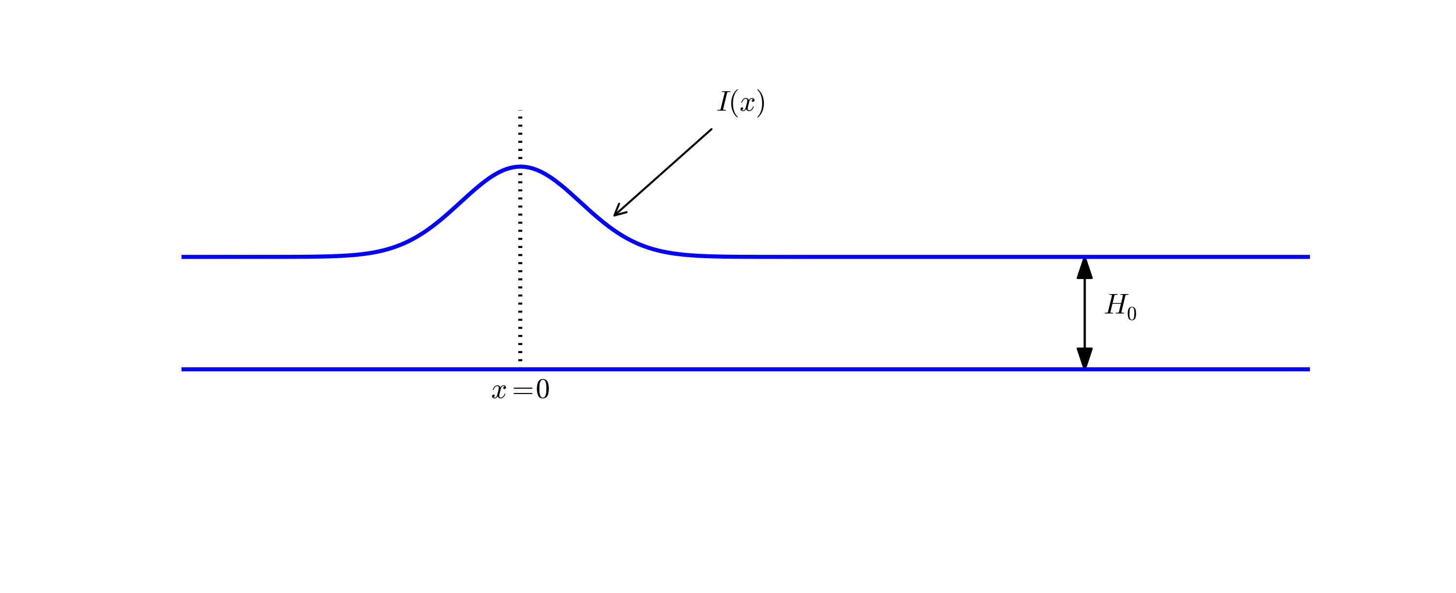
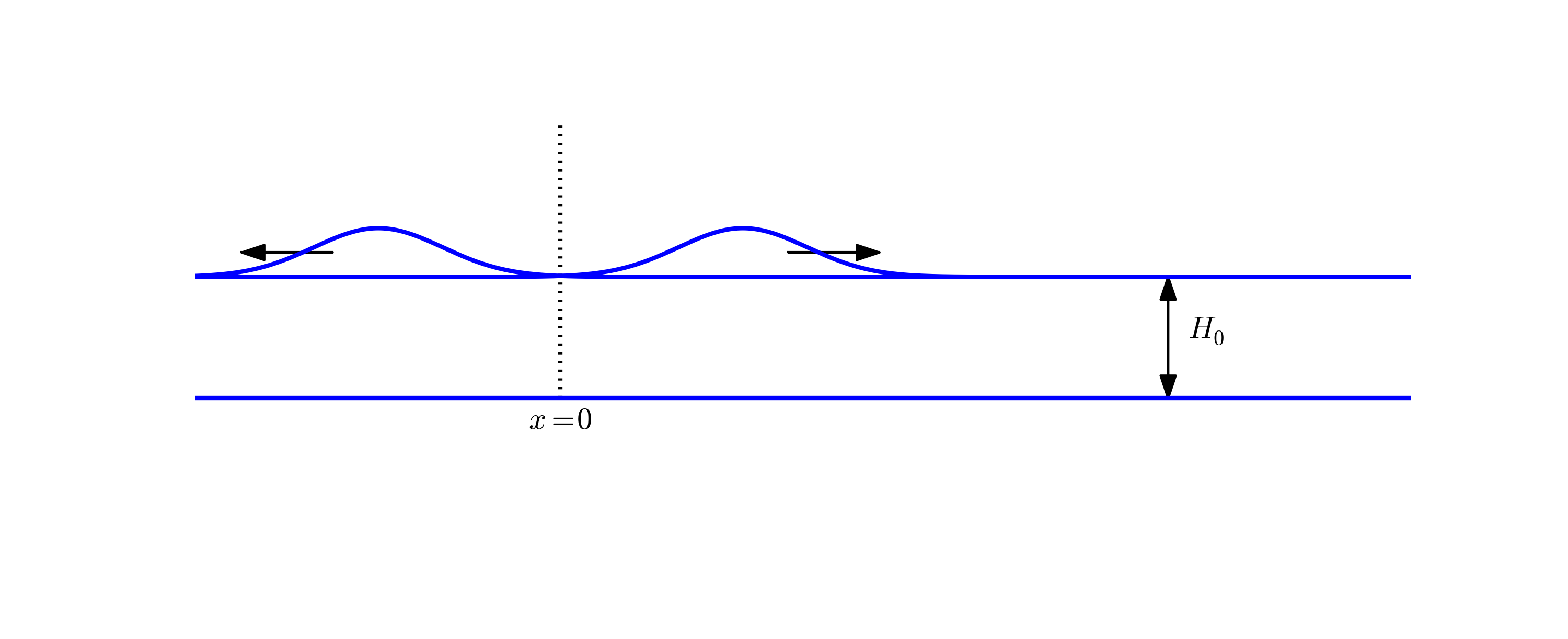
To simulate the right-going tsunami, we can impose a symmetry boundary at \(x=0\): \(\partial\eta/\partial x =0\). We then simulate the wave motion in \([0,L]\). Unless the ocean ends at \(x=L\), the waves should travel undisturbed through the boundary \(x=L\). A radiation condition as explained in Problem Section 2.36 can be used for this purpose. Alternatively, one can just stop the simulations before the wave hits the boundary at \(x=L\). In that case it does not matter what kind of boundary condition we use at \(x=L\). Imposing \(\eta =0\) and stopping the simulations when \(|\eta_i^n| > \epsilon\), \(i=N_x-1\), is a possibility (\(\epsilon\) is a small parameter).

The shape of the initial surface can be taken as a Gaussian function, \[ I(x;I_0,I_a,I_m,I_s) = I_0 + I_a\exp{\left(-\left(\frac{x-I_m}{I_s}\right)^2\right)}, \] with \(I_m=0\) reflecting the location of the peak of \(I(x)\) and \(I_s\) being a measure of the width of the function \(I(x)\) (\(I_s\) is \(\sqrt{2}\) times the standard deviation of the familiar normal distribution curve).

Now we extend the problem with a hill at the sea bottom, see Figure Figure 2.10. The wave speed \(c=\sqrt{gH(x)} = \sqrt{g(H_0-B(x))}\) will then be reduced in the shallow water above the hill.

Figure 2.10: Sketch of an earthquake-generated tsunami passing over a subsea hill.

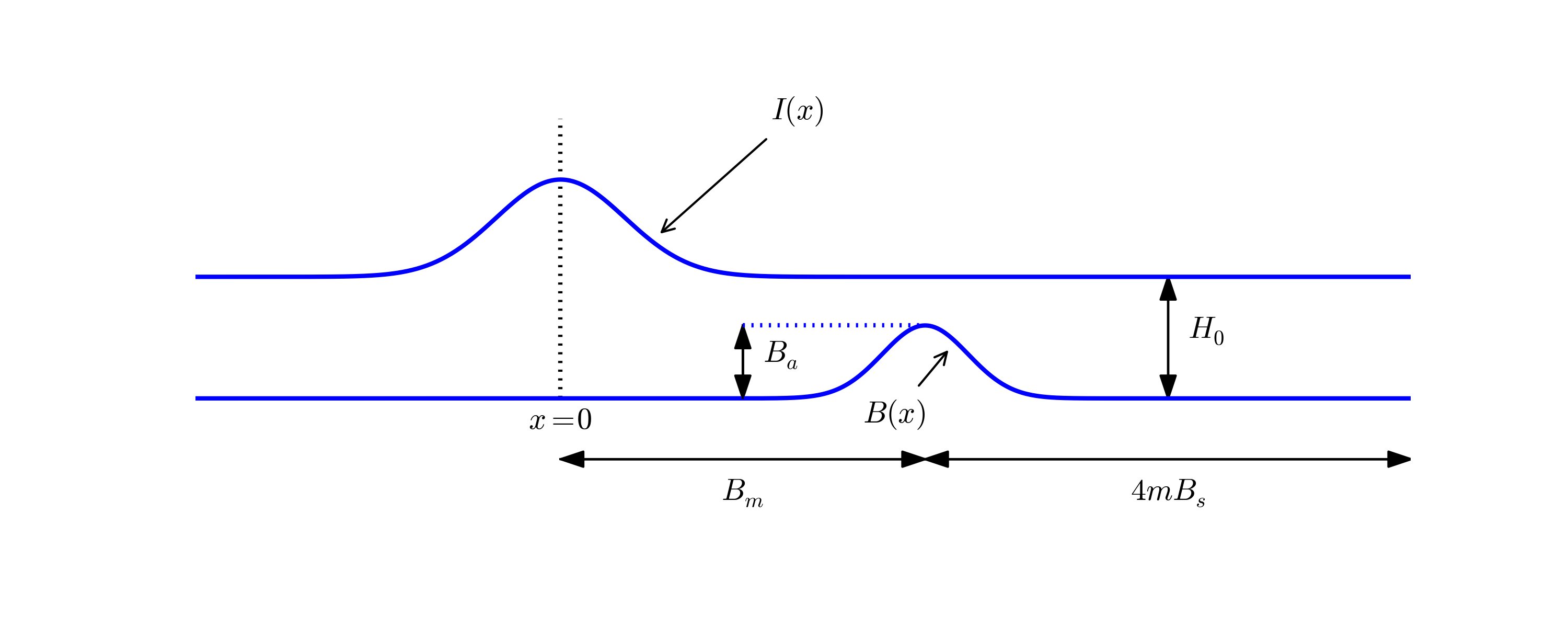
One possible form of the hill is a Gaussian function, \[ B(x;B_0,B_a,B_m,B_s) = B_0 + B_a\exp{\left(-\left(\frac{x-B_m}{B_s}\right)^2\right)}, \tag{2.115}\] but many other shapes are also possible, e.g., a “cosine hat” where \[ B(x; B_0, B_a, B_m, B_s) = B_0 + B_a\cos{\left( \pi\frac{x-B_m}{2B_s}\right)}, \tag{2.116}\] when \(x\in [B_m - B_s, B_m + B_s]\) while \(B=B_0\) outside this interval.

Also an abrupt construction may be tried: \[ B(x; B_0, B_a, B_m, B_s) = B_0 + B_a, \tag{2.117}\] for \(x\in [B_m - B_s, B_m + B_s]\) while \(B=B_0\) outside this interval.

The Devito solver from Section 2.12 can be used as a starting point for the implementation. Visualize both the bottom topography and the water surface elevation in the same plot. Allow for a flexible choice of bottom shape: (2.115), (2.116), (2.117), or \(B(x)=B_0\) (flat).

The purpose of this problem is to explore the quality of the numerical solution \(\eta^n_i\) for different shapes of the bottom obstruction. The “cosine hat” and the box-shaped hills have abrupt changes in the derivative of \(H(x)\) and are more likely to generate numerical noise than the smooth Gaussian shape of the hill. Investigate if this is true.

2.66 Problem: Earthquake-generated tsunami over a 3D hill

This problem extends Problem Section 2.65 to a three-dimensional wave phenomenon, governed by the 2D PDE \[ \eta_{tt} = (gH\eta_x)_x + (gH\eta_y)_y = \nabla\cdot (gH\nabla\eta) \tp \tag{2.118}\] We assume that the earthquake arises from a fault along the line \(x=0\) in the \(xy\)-plane so that the initial lift of the surface can be taken as \(I(x)\) in Problem Section 2.65. That is, a plane wave is propagating to the right, but will experience bending because of the bottom.

The bottom shape is now a function of \(x\) and \(y\). An “elliptic” Gaussian function in two dimensions, with its peak at \((B_{mx}, B_{my})\), generalizes (2.115): \[ B = B_0 + B_a\exp{\left(-\left(\frac{x-B_{mx}}{B_s}\right)^2 -\left(\frac{y-B_{my}}{bB_s}\right)^2\right)}, \tag{2.119}\] where \(b\) is a scaling parameter: \(b=1\) gives a circular Gaussian function with circular contour lines, while \(b\neq 1\) gives an elliptic shape with elliptic contour lines. To indicate the input parameters in the model, we may write \[ B = B(x;B_0,B_a,B_{mx}, B_{my} ,B_s, b)\tp \] The “cosine hat” (2.116) can also be generalized to \[ B = B_0 + B_a\cos{\left( \pi\frac{x-B_{mx}}{2B_s}\right)} \cos{\left( \pi\frac{y-B_{my}}{2B_s}\right)}, \tag{2.120}\] when \(0 \leq \sqrt{x^2+y^2} \leq B_s\) and \(B=B_0\) outside this circle.

A box-shaped obstacle means that \[ B(x; B_0, B_a, B_m, B_s, b) = B_0 + B_a \tag{2.121}\] for \(x\) and \(y\) inside a rectangle \[ B_{mx}-B_s \leq x \leq B_{mx} + B_s,\quad B_{my}-bB_s \leq y \leq B_{my} + bB_s, \] and \(B=B_0\) outside this rectangle. The \(b\) parameter controls the rectangular shape of the cross section of the box.

Note that the initial condition and the listed bottom shapes are symmetric around the line \(y=B_{my}\). We therefore expect the surface elevation also to be symmetric with respect to this line. This means that we can halve the computational domain by working with \([0,L_x]\times [0, B_{my}]\). Along the upper boundary, \(y=B_{my}\), we must impose the symmetry condition \(\partial \eta/\partial n=0\). Such a symmetry condition (\(-\eta_x=0\)) is also needed at the \(x=0\) boundary because the initial condition has a symmetry here. At the lower boundary \(y=0\) we also set a Neumann condition (which becomes \(-\eta_y=0\)). The wave motion is to be simulated until the wave hits the reflecting boundaries where \(\partial\eta/\partial n =\eta_x =0\) (one can also set \(\eta =0\) - the particular condition does not matter as long as the simulation is stopped before the wave is influenced by the boundary condition).

Visualize the surface elevation. Investigate how different hill shapes, different sizes of the water gap above the hill, and different resolutions \(\Delta x = \Delta y = h\) and \(\Delta t\) influence the numerical quality of the solution.

2.67 Problem: Investigate Mayavi for visualization

Play with Mayavi code for visualizing 2D solutions of the wave equation with variable wave velocity. See if there are effective ways to visualize both the solution and the wave velocity scalar field at the same time.

2.68 Problem: Investigate visualization packages

Create some fancy 3D visualization of the water waves and the subsea hill in Problem Section 2.66. Try to make the hill transparent. Possible visualization tools are Mayavi, Paraview, and OpenDX.

2.69 Problem: Implement loops in compiled languages

Extend the program from Problem Section 2.66 such that the loops over mesh points, inside the time loop, are implemented in compiled languages. Consider implementations in Cython, Fortran via f2py, C via Cython, C via f2py, C/C++ via Instant, and C/C++ via scipy.weave. Perform efficiency experiments to investigate the relative performance of the various implementations. It is often advantageous to normalize CPU times by the fastest method on a given mesh.

2.70 Exercise: Simulate seismic waves in 2D

The goal of this exercise is to simulate seismic waves using the PDE model (2.98) in a 2D \(xz\) domain with geological layers. Introduce \(m\) horizontal layers of thickness \(h_i\), \(i=0,\ldots,m-1\). Inside layer number \(i\) we have a vertical wave velocity \(c_{z,i}\) and a horizontal wave velocity \(c_{h,i}\). Make a program for simulating such 2D waves. Test it on a case with 3 layers where \[ c_{z,0}=c_{z,1}=c_{z,2},\quad c_{h,0}=c_{h,2},\quad c_{h,1} \ll c_{h,0} \tp \] Let \(s\) be a localized point source at the middle of the Earth’s surface (the upper boundary) and investigate how the resulting wave travels through the medium. The source can be a localized Gaussian peak that oscillates in time for some time interval. Place the boundaries far enough from the expanding wave so that the boundary conditions do not disturb the wave. Then the type of boundary condition does not matter, except that we physically need to have \(p=p_0\), where \(p_0\) is the atmospheric pressure, at the upper boundary.

2.71 Project: Model 3D acoustic waves in a room

The equation for sound waves in air is derived in Section Section 2.56 and reads \[ p_{tt} = c^2\nabla^2 p, \] where \(p(x,y,z,t)\) is the pressure and \(c\) is the speed of sound, taken as 340 m/s. However, sound is absorbed in the air due to relaxation of molecules in the gas. A model for simple relaxation, valid for gases consisting only of one type of molecules, is a term \(c^2\tau_s\nabla^2 p_t\) in the PDE, where \(\tau_s\) is the relaxation time. If we generate sound from, e.g., a loudspeaker in the room, this sound source must also be added to the governing equation.

The PDE with the mentioned type of damping and source then becomes \[ p_tt = c^2\nabla^p + c^2\tau_s\nabla^2 p_t + f, \] where \(f(x,y,z,t)\) is the source term.

The walls can absorb some sound. A possible model is to have a “wall layer” (thicker than the physical wall) outside the room where \(c\) is changed such that some of the wave energy is reflected and some is absorbed in the wall. The absorption of energy can be taken care of by adding a damping term \(bp_t\) in the equation: \[ p_tt + bp_t = c^2\nabla^p + c^2\tau_s\nabla^2 p_t + f\tp \] Typically, \(b=0\) in the room and \(b>0\) in the wall. A discontinuity in \(b\) or \(c\) will give rise to reflections. It can be wise to use a constant \(c\) in the wall to control reflections because of the discontinuity between \(c\) in the air and in the wall, while \(b\) is gradually increased as we go into the wall to avoid reflections because of rapid changes in \(b\). At the outer boundary of the wall the condition \(p=0\) or \(\partial p/\partial n=0\) can be imposed. The waves should anyway be approximately dampened to \(p=0\) this far out in the wall layer.

There are two strategies for discretizing the \(\nabla^2 p_t\) term: using a center difference between times \(n+1\) and \(n-1\) (if the equation is sampled at level \(n\)), or use a one-sided difference based on levels \(n\) and \(n-1\). The latter has the advantage of not leading to any equation system, while the former is second-order accurate as the scheme for the simple wave equation \(p_tt = c^2\nabla^2 p\). To avoid an equation system, go for the one-sided difference such that the overall scheme becomes explicit and only of first order in time.

Develop a 3D solver for the specified PDE and introduce a wall layer. Test the solver with the method of manufactured solutions. Make some demonstrations where the wall reflects and absorbs the waves (reflection because of discontinuity in \(b\) and absorption because of growing \(b\)). Experiment with the impact of the \(\tau_s\) parameter.

2.72 Project: Solve a 1D transport equation

We shall study the wave equation \[ u_t + cu_x = 0,\quad x\in (0,L],\ t\in (0, T], \tag{2.122}\] with initial condition \[ u(x,0) = I(x),\quad x\in [0,L], \] and one periodic boundary condition \[ u(0,t) = u(L,t) \tp \] This boundary condition means that what goes out of the domain at \(x=L\) comes in at \(x=0\). Roughly speaking, we need only one boundary condition because the spatial derivative is of first order only.

Physical interpretation. The parameter \(c\) can be constant or variable, \(c=c(x)\). The equation (2.122) arises in transport problems where a quantity \(u\), which could be temperature or concentration of some contaminant, is transported with the velocity \(c\) of a fluid. In addition to the transport imposed by ``travelling with the fluid’’, \(u\) may also be transported by diffusion (such as heat conduction or Fickian diffusion), but we have in the model \(u_t + cu_x\) assumed that diffusion effects are negligible, which they often are.

a)

Show that under the assumption of \(a=\text{const}\), \[ u(x,t) = I(x - ct) \tag{2.123}\] fulfills the PDE as well as the initial and boundary condition (provided \(I(0)=I(L)\)).

A widely used numerical scheme for (2.122) applies a forward difference in time and a backward difference in space when \(c>0\): \[ [D_t^+ u + cD_x^-u = 0]_i^n \tp \tag{2.124}\] For \(c<0\) we use a forward difference in space: \([cD_x^+u]_i^n\).

b)

Set up a computational algorithm and implement it in a function. Assume \(a\) is constant and positive.

c)

Test the implementation by using the remarkable property that the numerical solution is exact at the mesh points if \(\Delta t = c^{-1}\Delta x\).

d)

Make a movie comparing the numerical and exact solution for the following two choices of initial conditions: \[ I(x) = \left\lbrack\sin\left(\pi\frac{x}{L}\right)\right\rbrack^{2n} \tag{2.125}\] where \(n\) is an integer, typically \(n=5\), and \[ I(x) = \exp{\left( -\frac{(x-L/2)^2}{2\sigma2}\right)} \tp \tag{2.126}\] Choose \(\Delta t = c^{-1}\Delta x, 0.9c^{-1}\Delta x, 0.5c^{-1}\Delta x\).

e)

The performance of the suggested numerical scheme can be investigated by analyzing the numerical dispersion relation. Analytically, we have that the Fourier component \[ u(x,t) = e^{i(kx-\omega t)}, \] is a solution of the PDE if \(\omega = kc\). This is the analytical dispersion relation. A complete solution of the PDE can be built by adding up such Fourier components with different amplitudes, where the initial condition \(I\) determines the amplitudes. The solution \(u\) is then represented by a Fourier series.

A similar discrete Fourier component at \((x_p,t_n)\) is \[ u_p^q = e^{i(kp\Delta x -\tilde\omega n\Delta t)}, \] where in general \(\tilde\omega\) is a function of \(k\), \(\Delta t\), and \(\Delta x\), and differs from the exact \(\omega =kc\).

Insert the discrete Fourier component in the numerical scheme and derive an expression for \(\tilde\omega\), i.e., the discrete dispersion relation. Show in particular that if \(\Delta t/(c\Delta x)=1\), the discrete solution coincides with the exact solution at the mesh points, regardless of the mesh resolution (!). Show that if the stability condition \[ \frac{\Delta t}{c\Delta x}\leq 1, \] the discrete Fourier component cannot grow (i.e., \(\tilde\omega\) is real).

f)

Write a test for your implementation where you try to use information from the numerical dispersion relation.

We shall hereafter assume that \(c(x)>0\).

g)

Set up a computational algorithm for the variable coefficient case and implement it in a function. Make a test that the function works for constant \(a\).

h)

It can be shown that for an observer moving with velocity \(c(x)\), \(u\) is constant. This can be used to derive an exact solution when \(a\) varies with \(x\). Show first that \[ u(x,t) = f(C(x) - t), \tag{2.127}\] where \[ C'(x) = \frac{1}{c(x)}, \] is a solution of (2.122) for any differentiable function \(f\).

Solution

Let \(\xi = C(x) - t\). We have that \[ u_t = f'(\xi)(-1), \] while \[ u_x = f'(\xi)C'(x) = f'(\xi)\frac{1}{c(x)}, \] implying that \(au_x = f'(\xi)\). Then we have \(u_t + cu_x= -f'(\xi) + f'(\xi) = 0\).

i)

Use the initial condition to show that an exact solution is \[ u(x,t) = I(C^{-1}(C(x)-t)), \] with \(C^{-1}\) being the inverse function of \(C = \int c^{1}dx\). Since \(C(x)\) is an integral \(\int_0^x (1/c)dx\), \(C(x)\) is monotonically increasing and there exists hence an inverse function \(C^{-1}\) with values in \([0,L]\).

Solution

In general we have \(u(x,t) = f(C(x)-t)\) and the solution is of this form with \(f(\xi)=I(C^{-1}(\xi))\). Moreover, at \(t=0\) we have \(I(C^{-1}(C(x)))=I(x)\), which is the required initial condition.

To compute (2.127) we need to integrate \(1/c\) to obtain \(C\) and then compute the inverse of \(C\).

The inverse function computation can be easily done if we first think discretely. Say we have some function \(y=g(x)\) and seek its inverse. Plotting \((x_i,y_i)\), where \(y_i=g(x_i)\) for some mesh points \(x_i\), displays \(g\) as a function of \(x\). The inverse function is simply \(x\) as a function of \(g\), i.e., the curve with points \((y_i,x_i)\). We can therefore quickly compute points at the curve of the inverse function. One way of extending these points to a continuous function is to assume a linear variation (known as linear interpolation) between the points (which actually means to draw straight lines between the points, exactly as done by a plotting program).

The function scipy.interpolate.interp1d can take a set of points and return a continuous function that corresponds to linear variation between the points. The computation of the inverse of a function \(g\) on \([0,L]\) can then be done by

def inverse(g, domain, resolution=101):
    x = linspace(domain[0], domain[L], resolution)
    y = g(x)
    from scipy.interpolate import interp1d
    g_inverse = interp1d(y, x, kind='linear', fill_value='extrapolate')
    return g_inverse

To compute \(C(x)\) we need to integrate \(1/c\), which can be done by a Trapezoidal rule. Suppose we have computed \(C(x_i)\) and need to compute \(C(x_{i+1})\). Using the Trapezoidal rule with \(m\) subintervals over the integration domain \([x_i,x_{i+1}]\) gives \[ C(x_{i+1}) = C(x_i) + \int_{x_i}^{x_{i+1}} \frac{dx}{c} \approx h\left( \half\frac{1}{c(x_i)} + \half\frac{1}{c(x_{i+1})} + \sum_{j=1}^{m-1} \frac{1}{c(x_i + jh)}\right), \tag{2.128}\] where \(h=(x_{i+1}-x_i)/m\) is the length of the subintervals used for the integral over \([x_i,x_{i+1}]\). We observe that (2.128) is a difference equation which we can solve by repeatedly applying (2.128) for \(i=0,1,\ldots,N_x-1\) if a mesh \(x_0,x_,\ldots,x_{N_x}\) is prescribed. Note that \(C(0)=0\).

j)

Implement a function for computing \(C(x_i)\) and one for computing \(C^{-1}(x)\) for any \(x\). Use these two functions for computing the exact solution \(I(C^{-1}(C(x)-t))\). End up with a function u_exact_variable_c(x, n, c, I) that returns the value of \(I(C^{-1}(C(x)-t_n))\).

k)

Make movies showing a comparison of the numerical and exact solutions for the two initial conditions (1) and (2.126). Choose \(\Delta t = \Delta x /\max_{0,L} c(x)\) and the velocity of the medium as

1. \(c(x) = 1 + \epsilon\sin(k\pi x/L)\), \(\epsilon <1\),
2. \(c(x) = 1 + I(x)\), where \(I\) is given by

1. or (2.126).

The PDE \(u_t + cu_x=0\) expresses that the initial condition \(I(x)\) is transported with velocity \(c(x)\).

2.73 Problem: General analytical solution of a 1D damped wave equation

2.74 For solution, see damped_wave_equation.pdf in joakibo on bitbucket.

We consider an initial-boundary value problem for the damped wave equation:

\[\begin{alignat*}{2} u_{tt} +bu_t &= c^2 u_{xx}, \quad &x\in (0,L),\ t\in (0,T]\\ u(0,t) &= 0,\\ u(L,t) &=0,\\ u(x, 0) &= I(x),\\ u_t(x, 0) &= V(x)\tp \end{alignat*}\] Here, \(b\geq 0\) and \(c\) are given constants. The aim is to derive a general analytical solution of this problem. Familiarity with the method of separation of variables for solving PDEs will be assumed.

a)

Seek a solution on the form \(u(x,t)=X(x)T(t)\). Insert this solution in the PDE and show that it leads to two differential equations for \(X\) and \(T\): \[ T'' + bT' + \lambda T = 0,\quad c^2 X'' +\lambda X = 0, \] with \(X(0)=X(L)=0\) as boundary conditions, and \(\lambda\) as a constant to be determined.

b)

Show that \(X(x)\) is on the form \[ X_n(x) = C_n\sin kx,\quad k = \frac{n\pi}{L},\quad n=1,2,\ldots \] where \(C_n\) is an arbitrary constant.

c)

Under the assumption that \((b/2)^2 < k^2\), show that \(T(t)\) is on the form \[ T_n(t) = e^{-{\half}bt}(a_n\cos\omega t + b_n\sin\omega t), \quad\omega = \sqrt{k^2 - \frac{1}{4}b^2},\quad n=1,2,\ldots \] The complete solution is then \[ u(x,t) = \sum_{n=1}^\infty \sin kx e^{-{\half}bt}( A_n\cos\omega t + B_n\sin\omega t), \] where the constants \(A_n\) and \(B_n\) must be computed from the initial conditions.

d)

Derive a formula for \(A_n\) from \(u(x,0)=I(x)\) and developing \(I(x)\) as a sine Fourier series on \([0,L]\).

e)

Derive a formula for \(B_n\) from \(u_t(x,0)=V(x)\) and developing \(V(x)\) as a sine Fourier series on \([0,L]\).

f)

Calculate \(A_n\) and \(B_n\) from vibrations of a string where \(V(x)=0\) and \[ I(x) = \left\lbrace \begin{array}{ll} ax/x_0, & x < x_0,\\ a(L-x)/(L-x_0), & \text{otherwise} \end{array}\right. \]

g)

Implement a function u_series(x, t, tol=1E-10) for the series for \(u(x,t)\), where tol is a tolerance for truncating the series. Simply sum the terms until \(|a_n|\) and \(|b_b|\) both are less than tol.

h)

What will change in the derivation of the analytical solution if we have \(u_x(0,t)=u_x(L,t)=0\) as boundary conditions? And how will you solve the problem with \(u(0,t)=0\) and \(u_x(L,t)=0\)?

2.75 Problem: General analytical solution of a 2D damped wave equation

Carry out Problem Section 2.73 in the 2D case: \(u_{tt}+bu_t = c^2(u_{xx}+u_{yy})\), where \((x,y)\in (0,L_x)\times (0,L_y)\). Assume a solution on the form \(u(x,y,t)=X(x)Y(y)T(t)\).

2.76 Exercises: Wave Equations with Devito

These exercises explore wave equation solutions using the Devito DSL. They progress from basic usage through verification techniques to more advanced applications.

2.76.1 Exercise 1: Standing Wave Simulation

Use the solve_wave_1d function to simulate a standing wave with:

• Domain: \(L = 1\), wave speed \(c = 1\)
• Initial condition: \(I(x) = \sin(2\pi x)\) (two half-wavelengths)
• Initial velocity: \(V = 0\)
• Boundary conditions: \(u(0, t) = u(1, t) = 0\)

a) Compute and plot the solution at \(t = 0, 0.25, 0.5, 0.75, 1.0\). How does the pattern differ from the fundamental mode?

b) Derive the exact solution for this initial condition and compare with the numerical solution. Compute the maximum error at \(t = 1\) for \(N_x = 50, 100, 200\).

Solution

from src.wave import solve_wave_1d, exact_standing_wave
import numpy as np
import matplotlib.pyplot as plt

# Part (a)
def I(x):
    return np.sin(2 * np.pi * x)

times = [0, 0.25, 0.5, 0.75, 1.0]
fig, axes = plt.subplots(1, 5, figsize=(15, 3))

for ax, T in zip(axes, times):
    result = solve_wave_1d(L=1.0, c=1.0, Nx=100, T=T, C=0.9, I=I)
    ax.plot(result.x, result.u)
    ax.set_title(f't = {T}')
    ax.set_ylim(-1.2, 1.2)

plt.tight_layout()

# Part (b) - The exact solution for m=2 mode
# u(x,t) = sin(2*pi*x) * cos(2*pi*t)
def u_exact(x, t):
    return np.sin(2 * np.pi * x) * np.cos(2 * np.pi * t)

for Nx in [50, 100, 200]:
    result = solve_wave_1d(L=1.0, c=1.0, Nx=Nx, T=1.0, C=0.9, I=I)
    error = np.abs(result.u - u_exact(result.x, 1.0)).max()
    print(f"Nx = {Nx:3d}: max error = {error:.2e}")

2.76.2 Exercise 2: Convergence Rate Verification

The theoretical convergence rate for the wave equation solver is \(O(\Delta t^2 + \Delta x^2) = O(h^2)\) when \(\Delta t \propto \Delta x\).

a) Use convergence_test_wave_1d with grid sizes \(N_x = 20, 40, 80, 160, 320\) and verify the observed rate is close to 2.

b) Repeat with Courant number \(C = 1\). What happens to the errors? Explain why.

Solution

from src.wave import convergence_test_wave_1d
import numpy as np

# Part (a)
grid_sizes, errors, rate = convergence_test_wave_1d(
    grid_sizes=[20, 40, 80, 160, 320],
    T=0.5,
    C=0.9,
)
print(f"C = 0.9: Observed rate = {rate:.3f}")

# Compute individual rates
for i in range(1, len(errors)):
    r = np.log(errors[i-1] / errors[i]) / np.log(2)
    print(f"  Nx {grid_sizes[i-1]} -> {grid_sizes[i]}: rate = {r:.3f}")

# Part (b)
grid_sizes, errors, rate = convergence_test_wave_1d(
    grid_sizes=[20, 40, 80, 160, 320],
    T=0.5,
    C=1.0,
)
print(f"\nC = 1.0: Observed rate = {rate:.3f}")
print(f"Errors: {errors}")

# At C=1, the numerical method is exact for the standing wave!
# Errors should be near machine precision.

2.76.3 Exercise 3: Guitar String

Simulate a plucked guitar string with a triangular initial shape: \[ I(x) = \begin{cases} ax/x_0 & x < x_0 \\ a(L-x)/(L-x_0) & x \ge x_0 \end{cases} \]

where \(L = 0.75\) m, \(x_0 = 0.8L\), and \(a = 0.005\) m.

a) For a guitar with fundamental frequency 440 Hz, compute the wave speed \(c\) given that \(\lambda = 2L\).

b) Simulate one complete period and create an animation. Does the triangular shape remain sharp as time progresses?

c) Run with \(C = 1\) and observe the difference. Explain why the result is different.

Solution

from src.wave import solve_wave_1d
import numpy as np

# Parameters
L = 0.75
x0 = 0.8 * L
a = 0.005
freq = 440  # Hz

# Part (a)
wavelength = 2 * L
c = freq * wavelength
print(f"Wave speed c = {c} m/s")

# Period
period = 1 / freq
print(f"Period = {period*1000:.3f} ms")

# Part (b)
def I(x):
    return np.where(x < x0, a * x / x0, a * (L - x) / (L - x0))

result = solve_wave_1d(
    L=L, c=c, Nx=150, T=period,
    C=0.9, I=I, save_history=True
)

# The triangular shape becomes "wavy" due to numerical dispersion
# Different Fourier components travel at slightly different speeds

# Part (c)
result_exact = solve_wave_1d(
    L=L, c=c, Nx=150, T=period,
    C=1.0, I=I, save_history=True
)

# At C=1, D'Alembert's solution is exactly reproduced:
# The triangular pulse splits into two, bounces off walls, and
# recombines after one period to give the original shape.

2.76.4 Exercise 4: Source Wavelets

a) Use ricker_wavelet to create wavelets with peak frequencies \(f_0 = 10, 25, 50\) Hz. Plot them and their frequency spectra.

b) What is the relationship between \(f_0\) and the dominant wavelength \(\lambda\) in a medium with \(c = 1500\) m/s?

c) For seismic imaging, we typically want the wavelet to have negligible amplitude at \(t = 0\). What constraint does this place on \(t_0\) relative to \(f_0\)?

Solution

from src.wave import ricker_wavelet, get_source_spectrum
import numpy as np
import matplotlib.pyplot as plt

# Part (a)
t = np.linspace(0, 0.5, 1001)
dt = t[1] - t[0]

fig, axes = plt.subplots(2, 3, figsize=(12, 6))

for i, f0 in enumerate([10, 25, 50]):
    wavelet = ricker_wavelet(t, f0=f0)
    freq, amp = get_source_spectrum(wavelet, dt)

    axes[0, i].plot(t, wavelet)
    axes[0, i].set_title(f'f0 = {f0} Hz')
    axes[0, i].set_xlabel('Time (s)')

    axes[1, i].plot(freq[:100], amp[:100])
    axes[1, i].axvline(f0, color='r', linestyle='--')
    axes[1, i].set_xlabel('Frequency (Hz)')

# Part (b)
c = 1500  # m/s
for f0 in [10, 25, 50]:
    wavelength = c / f0
    print(f"f0 = {f0} Hz: wavelength = {wavelength} m")

# Part (c)
# The Ricker wavelet is centered at t0, and has amplitude ~0 when
# |t - t0| > 1/f0. For the wavelet to be ~0 at t=0, we need:
# t0 > 1/f0, typically t0 = 1.5/f0 is used as default

2.76.5 Exercise 5: 2D Wave Propagation

a) Solve the 2D wave equation with an initial Gaussian pulse centered at \((0.5, 0.5)\): \[ I(x, y) = e^{-100((x-0.5)^2 + (y-0.5)^2)} \]

Plot the solution at \(t = 0, 0.1, 0.2, 0.3\) using contour plots.

b) How does the wave pattern differ from the 1D case? Explain the amplitude decay you observe.

Solution

from src.wave import solve_wave_2d
import numpy as np
import matplotlib.pyplot as plt

# Part (a)
def I(X, Y):
    return np.exp(-100 * ((X - 0.5)**2 + (Y - 0.5)**2))

fig, axes = plt.subplots(1, 4, figsize=(16, 4))

for ax, T in zip(axes, [0, 0.1, 0.2, 0.3]):
    result = solve_wave_2d(
        Lx=1.0, Ly=1.0, Nx=100, Ny=100,
        T=T, C=0.5, I=I
    )

    X, Y = np.meshgrid(result.x, result.y, indexing='ij')
    c = ax.contourf(X, Y, result.u, levels=20, cmap='RdBu_r')
    ax.set_title(f't = {T}')
    ax.set_aspect('equal')

# Part (b)
# In 2D, the wave spreads as a circular wavefront. The amplitude
# decays as 1/sqrt(r) due to geometric spreading - the energy is
# distributed over an expanding circle rather than staying constant
# as in 1D.

2.76.6 Exercise 6: Reflection from Interface

Consider a 1D domain \([0, 2]\) with a velocity interface at \(x = 1\): \(c(x) = 1\) for \(x < 1\) and \(c(x) = 2\) for \(x \ge 1\).

a) Starting with a Gaussian pulse centered at \(x = 0.3\), simulate the wave propagation until \(t = 2.0\).

b) Identify the reflected and transmitted waves. Do the amplitudes match the theoretical reflection (\(R = 1/3\)) and transmission (\(T = 4/3\)) coefficients?

c) What happens at the boundaries \(x = 0\) and \(x = 2\)? Are there additional reflections?

Solution

# This requires implementing variable velocity, which is
# demonstrated in the wave1D_features.qmd chapter.
# A simplified approach using manual stencil computation:

import numpy as np
import matplotlib.pyplot as plt

L = 2.0
Nx = 400
dx = L / Nx
x = np.linspace(0, L, Nx + 1)

# Velocity profile
c = np.where(x < 1.0, 1.0, 2.0)
c_max = 2.0

# Time stepping
C = 0.5
dt = C * dx / c_max
T = 2.0
Nt = int(T / dt)

# Initial condition
sigma = 0.1
x0 = 0.3
u_nm1 = np.exp(-((x - x0) / sigma)**2)
u_n = u_nm1.copy()
u = np.zeros_like(u_n)

# Store snapshots
snapshots = []
times = []

for n in range(Nt):
    # Update interior
    for i in range(1, Nx):
        C_local = c[i] * dt / dx
        u[i] = 2*u_n[i] - u_nm1[i] + C_local**2 * (u_n[i+1] - 2*u_n[i] + u_n[i-1])

    # Dirichlet BCs
    u[0] = 0
    u[Nx] = 0

    # Swap
    u_nm1, u_n, u = u_n, u, u_nm1

    # Store snapshots
    if n % 50 == 0:
        snapshots.append(u_n.copy())
        times.append(n * dt)

# Plot snapshots
fig, axes = plt.subplots(2, 4, figsize=(16, 6))
for ax, snap, t in zip(axes.flat, snapshots, times):
    ax.plot(x, snap)
    ax.axvline(1.0, color='gray', linestyle='--', label='interface')
    ax.set_ylim(-1, 1)
    ax.set_title(f't = {t:.2f}')

2.76.7 Exercise 7: Manufactured Solution

Use the method of manufactured solutions to verify the solver. Choose \(u(x, t) = x(L-x)(1 + t/2)\) which satisfies zero Dirichlet boundary conditions.

a) Compute the required source term \(f(x, t)\) and initial conditions \(I(x)\), \(V(x)\).

b) Modify the solver (or use the source term capability) to solve with this \(f(x, t)\). Verify the numerical solution matches the exact solution to machine precision.

Solution

# Manufactured solution: u = x(L-x)(1 + t/2)
# u_t = x(L-x) * (1/2)
# u_tt = 0
# u_x = (L - 2x)(1 + t/2)
# u_xx = -2(1 + t/2)
#
# PDE: u_tt = c^2 * u_xx + f
# 0 = c^2 * (-2)(1 + t/2) + f
# f = 2*c^2*(1 + t/2)

L = 2.5
c = 1.5

def u_exact(x, t):
    return x * (L - x) * (1 + 0.5 * t)

def I(x):
    return u_exact(x, 0)

def V(x):
    return 0.5 * x * (L - x)

def f(x, t):
    return 2 * c**2 * (1 + 0.5 * t)

# The solution should be exact to machine precision because
# the discretization error is zero for quadratic solutions

2.76.8 Exercise 8: Wave Energy Conservation

The total energy of the wave system is: \[ E = \frac{1}{2} \int_0^L \left[ u_t^2 + c^2 u_x^2 \right] dx \]

a) Implement a function to compute the discrete energy at each time step.

b) Run a simulation with zero Dirichlet BCs and plot the energy versus time. Is energy conserved?

c) What happens to energy conservation if \(C > 1\)?

Solution

from src.wave import solve_wave_1d
import numpy as np

def compute_energy(u_history, x, dt, c):
    """Compute discrete energy at each time step."""
    dx = x[1] - x[0]
    Nt = u_history.shape[0]
    energy = np.zeros(Nt)

    for n in range(1, Nt-1):
        # u_t approximation (central difference)
        u_t = (u_history[n+1] - u_history[n-1]) / (2 * dt)

        # u_x approximation
        u_x = np.zeros_like(u_history[n])
        u_x[1:-1] = (u_history[n, 2:] - u_history[n, :-2]) / (2 * dx)

        # Energy integral
        energy[n] = 0.5 * dx * np.sum(u_t**2 + c**2 * u_x**2)

    return energy

# Part (b)
result = solve_wave_1d(
    L=1.0, c=1.0, Nx=100, T=5.0, C=0.9,
    save_history=True
)

E = compute_energy(result.u_history, result.x, result.dt, 1.0)

import matplotlib.pyplot as plt
plt.plot(result.t_history[1:-1], E[1:-1])
plt.xlabel('Time')
plt.ylabel('Energy')
plt.title('Energy Conservation')
# Energy should be nearly constant for stable schemes

# Part (c)
# For C > 1, the scheme is unstable and energy grows exponentially

2.76.9 Exercise 9: Numerical Dispersion

The numerical scheme introduces dispersion: different frequencies travel at different speeds.

a) Create an initial condition with multiple frequencies: \[ I(x) = \sin(2\pi x) + 0.5 \sin(6\pi x) \]

Simulate for several periods and observe how the shape changes.

b) Run the same simulation with \(C = 1\). Is dispersion present?

Solution

from src.wave import solve_wave_1d
import numpy as np
import matplotlib.pyplot as plt

def I(x):
    return np.sin(2 * np.pi * x) + 0.5 * np.sin(6 * np.pi * x)

# Part (a) - C < 1: dispersion present
result_a = solve_wave_1d(
    L=1.0, c=1.0, Nx=100, T=10.0, C=0.8,
    I=I, save_history=True
)

# Part (b) - C = 1: no dispersion
result_b = solve_wave_1d(
    L=1.0, c=1.0, Nx=100, T=10.0, C=1.0,
    I=I, save_history=True
)

# Compare at final time
fig, (ax1, ax2) = plt.subplots(1, 2, figsize=(12, 4))

ax1.plot(result_a.x, I(result_a.x), 'k--', label='Initial')
ax1.plot(result_a.x, result_a.u, 'r-', label=f't = {result_a.t}')
ax1.set_title('C = 0.8 (dispersion present)')
ax1.legend()

ax2.plot(result_b.x, I(result_b.x), 'k--', label='Initial')
ax2.plot(result_b.x, result_b.u, 'r-', label=f't = {result_b.t}')
ax2.set_title('C = 1.0 (dispersion-free)')
ax2.legend()

# At C = 1, the solution returns exactly to the initial shape
# after one period, while at C < 1, the shape is distorted.

2.76.10 Exercise 10: Extension to Higher Order

Devito supports higher-order spatial discretization through the space_order parameter.

a) Compare the errors at \(t = 1\) for space_order = 2, 4, 6, 8 with \(N_x = 50\).

b) For which problems might higher spatial order be beneficial?

Solution

# Note: This requires modifying the solver to accept space_order
# as a parameter. The key change is:
#
# u = TimeFunction(name='u', grid=grid, time_order=2, space_order=order)
#
# Higher order gives more accurate spatial derivatives but
# requires wider stencils and more boundary handling.
#
# Higher order is beneficial when:
# 1. The solution is smooth
# 2. Long propagation distances are needed
# 3. Minimizing numerical dispersion is important
# 4. Fewer grid points are desired for a given accuracy

Berenger, J.-P. 1994. “A Perfectly Matched Layer for the Absorption of Electromagnetic Waves.” Journal of Computational Physics 114: 185–200. https://doi.org/10.1006/jcph.1994.1159.

Cerjan, C., D. Kosloff, R. Kosloff, and M. Reshef. 1985. “A Nonreflecting Boundary Condition for Discrete Acoustic and Elastic Wave Equations.” Geophysics 50 (4): 705–8. https://doi.org/10.1190/1.1441945.

Clayton, R., and B. Engquist. 1977. “Absorbing Boundary Conditions for Acoustic and Elastic Wave Equations.” Bulletin of the Seismological Society of America 67 (6): 1529–40.

Dolci, D. I., E. M. Schliemann, L. F. Souza, et al. 2022. “Effectiveness and Computational Efficiency of Absorbing Boundary Conditions for Full-Waveform Inversion.” Geoscientific Model Development 15: 4077–99. https://doi.org/10.5194/gmd-15-5857-2022.

Engquist, B., and A. Majda. 1977. “Absorbing Boundary Conditions for the Numerical Simulation of Waves.” Mathematics of Computation 31: 629–51. https://doi.org/10.1090/S0025-5718-1977-0436612-4.

Grote, M. J., and I. Sim. 2010. “Efficient PML for the Wave Equation.” arXiv Preprint arXiv:1001.0319. https://arxiv.org/abs/1001.0319.

Higdon, R. L. 1986. “Absorbing Boundary Conditions for Difference Approximations to the Multi-Dimensional Wave Equation.” Mathematics of Computation 47 (176): 437–59. https://doi.org/10.1090/S0025-5718-1986-0856696-4.

———. 1987. “Numerical Absorbing Boundary Conditions for the Wave Equation.” Mathematics of Computation 49 (179): 65–90. https://doi.org/10.1090/S0025-5718-1987-0890254-1.

Langtangen, H. P. 2016. Finite Difference Computing with Exponential Decay Models. Lecture Notes in Computational Science and Engineering. Springer. http://hplgit.github.io/decay-book/doc/web/.

LeVeque, R. 2007. Finite Difference Methods for Ordinary and Partial Differential Equations: Steady-State and Time-Dependent Problems. SIAM.

Liu, Y., and M. K. Sen. 2018. “Hybrid Absorbing Boundary Condition for Piecewise Smooth Curved Boundary in 2D Acoustic Finite Difference Modelling.” Exploration Geophysics 49 (4): 469–83. https://doi.org/10.1071/EG17012.

Louboutin, Mathias, Michael Lange, Fabio Luporini, Navjot Kukreja, Philipp A. Witte, Felix J. Herrmann, Paulius Velesko, and Gerard J. Gorman. 2019. “Devito (v3.1.0): An Embedded Domain-Specific Language for Finite Differences and Geophysical Exploration.” Geoscientific Model Development 12: 1165–87. https://doi.org/10.5194/gmd-12-1165-2019.

Roden, J. A., and S. D. Gedney. 2000. “Convolution PML (CPML): An Efficient FDTD Implementation of the CFS-PML for Arbitrary Media.” Microwave and Optical Technology Letters 27 (5): 334–39. https://doi.org/10.1002/1098-2760(20001205)27:5<334::AID-MOP14>3.0.CO;2-A.

Sochacki, J., R. Kubichek, J. George, W. R. Fletcher, and S. Smithson. 1987. “Absorbing Boundary Conditions and Surface Waves.” Geophysics 52 (1): 60–71. https://doi.org/10.1190/1.1442241.

Strikwerda, J. 2007. Numerical Solution of Partial Differential Equations in Science and Engineering. Second. SIAM.