5 Nonlinear Problems
5.1 Linear versus nonlinear equations
5.1.1 Algebraic equations
A linear, scalar, algebraic equation in \(x\) has the form \[ ax + b = 0, \] for arbitrary real constants \(a\) and \(b\). The unknown is a number \(x\). All other algebraic equations, e.g., \(x^2 + ax + b = 0\), are nonlinear. The typical feature in a nonlinear algebraic equation is that the unknown appears in products with itself, like \(x^2\) or \(e^x = 1 + x +\half x^2 + \frac{1}{3!}x^3 + \cdots\).
We know how to solve a linear algebraic equation, \(x=-b/a\), but there are no general methods for finding the exact solutions of nonlinear algebraic equations, except for very special cases (quadratic equations constitute a primary example). A nonlinear algebraic equation may have no solution, one solution, or many solutions. The tools for solving nonlinear algebraic equations are iterative methods, where we construct a series of linear equations, which we know how to solve, and hope that the solutions of the linear equations converge to a solution of the nonlinear equation we want to solve. Typical methods for nonlinear algebraic equation equations are Newton’s method, the Bisection method, and the Secant method (Kelley 1995; Grief and Ascher 2011).
5.1.2 Differential equations
The unknown in a differential equation is a function and not a number. In a linear differential equation, all terms involving the unknown function are linear in the unknown function or its derivatives. Linear here means that the unknown function, or a derivative of it, is multiplied by a number or a known function. All other differential equations are non-linear.
The easiest way to see if an equation is nonlinear, is to spot nonlinear terms where the unknown function or its derivatives are multiplied by each other. For example, in \[ u^{\prime}(t) = -a(t)u(t) + b(t), \] the terms involving the unknown function \(u\) are linear: \(u^{\prime}\) contains the derivative of the unknown function multiplied by unity, and \(au\) contains the unknown function multiplied by a known function. However, \[ u^{\prime}(t) = u(t)(1 - u(t)), \] is nonlinear because of the term \(-u^2\) where the unknown function is multiplied by itself. Also \[ \frac{\partial u}{\partial t} + u\frac{\partial u}{\partial x} = 0, \] is nonlinear because of the term \(uu_x\) where the unknown function appears in a product with its derivative. (Note here that we use different notations for derivatives: \(u^{\prime}\) or \(du/dt\) for a function \(u(t)\) of one variable, \(\frac{\partial u}{\partial t}\) or \(u_t\) for a function of more than one variable.)
Another example of a nonlinear equation is \[ u^{\prime\prime} + \sin(u) =0, \] because \(\sin(u)\) contains products of \(u\), which becomes clear if we expand the function in a Taylor series: \[ \sin(u) = u - \frac{1}{3} u^3 + \ldots \]
To really prove mathematically that some differential equation in an unknown \(u\) is linear, show for each term \(T(u)\) that with \(u = au_1 + bu_2\) for constants \(a\) and \(b\), \[ T(au_1 + bu_2) = aT(u_1) + bT(u_2)\tp \] For example, the term \(T(u) = (\sin^2 t)u'(t)\) is linear because
\[\begin{align*} T(au_1 + bu_2) &= (\sin^2 t)(au_1(t) + b u_2(t))\\ & = a(\sin^2 t)u_1(t) + b(\sin^2 t)u_2(t)\\ & =aT(u_1) + bT(u_2)\tp \end{align*}\] However, \(T(u)=\sin u\) is nonlinear because \[ T(au_1 + bu_2) = \sin (au_1 + bu_2) \neq a\sin u_1 + b\sin u_2\tp \]
5.2 A simple model problem
A series of forthcoming examples will explain how to tackle nonlinear differential equations with various techniques. We start with the (scaled) logistic equation as model problem: \[ u^{\prime}(t) = u(t)(1 - u(t)) \tp \tag{5.1}\] This is a nonlinear ordinary differential equation (ODE) which will be solved by different strategies in the following. Depending on the chosen time discretization of (5.1), the mathematical problem to be solved at every time level will either be a linear algebraic equation or a nonlinear algebraic equation. In the former case, the time discretization method transforms the nonlinear ODE into linear subproblems at each time level, and the solution is straightforward to find since linear algebraic equations are easy to solve. However, when the time discretization leads to nonlinear algebraic equations, we cannot (except in very rare cases) solve these without turning to approximate, iterative solution methods.
The next subsections introduce various methods for solving nonlinear differential equations, using (5.1) as model. We shall go through the following set of cases:
- explicit time discretization methods (with no need to solve nonlinear algebraic equations)
- implicit Backward Euler time discretization, leading to nonlinear algebraic equations solved by
- an exact analytical technique
- Picard iteration based on manual linearization
- a single Picard step
- Newton’s method
- implicit Crank-Nicolson time discretization and linearization via a geometric mean formula
Thereafter, we compare the performance of the various approaches. Despite the simplicity of (5.1), the conclusions reveal typical features of the various methods in much more complicated nonlinear PDE problems.
5.3 Linearization by explicit time discretization
Time discretization methods are divided into explicit and implicit methods. Explicit methods lead to a closed-form formula for finding new values of the unknowns, while implicit methods give a linear or nonlinear system of equations that couples (all) the unknowns at a new time level. Here we shall demonstrate that explicit methods constitute an efficient way to deal with nonlinear differential equations.
The Forward Euler method is an explicit method. When applied to (5.1), sampled at \(t=t_n\), it results in \[ \frac{u^{n+1} - u^n}{\Delta t} = u^n(1 - u^n), \] which is a linear algebraic equation for the unknown value \(u^{n+1}\) that we can easily solve: \[ u^{n+1} = u^n + \Delta t\,u^n(1 - u^n)\tp \] In this case, the nonlinearity in the original equation poses no difficulty in the discrete algebraic equation. Any other explicit scheme in time will also give only linear algebraic equations to solve. For example, a typical 2nd-order Runge-Kutta method for (5.1) leads to the following formulas:
\[\begin{align*} u^* &= u^n + \Delta t u^n(1 - u^n),\\ u^{n+1} &= u^n + \Delta t \half \left( u^n(1 - u^n) + u^*(1 - u^*)) \right)\tp \end{align*}\] The first step is linear in the unknown \(u^*\). Then \(u^*\) is known in the next step, which is linear in the unknown \(u^{n+1}\) .
5.4 Exact solution of nonlinear algebraic equations
Switching to a Backward Euler scheme for (5.1), \[ \frac{u^{n} - u^{n-1}}{\Delta t} = u^n(1 - u^n), \tag{5.2}\] results in a nonlinear algebraic equation for the unknown value \(u^n\). The equation is of quadratic type: \[ \Delta t (u^n)^2 + (1-\Delta t)u^n - u^{n-1} = 0, \] and may be solved exactly by the well-known formula for such equations. Before we do so, however, we will introduce a shorter, and often cleaner, notation for nonlinear algebraic equations at a given time level. The notation is inspired by the natural notation (i.e., variable names) used in a program, especially in more advanced partial differential equation problems. The unknown in the algebraic equation is denoted by \(u\), while \(u^{(1)}\) is the value of the unknown at the previous time level (in general, \(u^{(\ell)}\) is the value of the unknown \(\ell\) levels back in time). The notation will be frequently used in later sections. What is meant by \(u\) should be evident from the context: \(u\) may either be 1) the exact solution of the ODE/PDE problem, 2) the numerical approximation to the exact solution, or 3) the unknown solution at a certain time level.
The quadratic equation for the unknown \(u^n\) in (5.2) can, with the new notation, be written \[ F(u) = \Delta t u^2 + (1-\Delta t)u - u^{(1)} = 0\tp \tag{5.3}\] The solution is readily found to be \[ u = \frac{1}{2\Delta t} \left(-1+\Delta t \pm \sqrt{(1-\Delta t)^2 - 4\Delta t u^{(1)}}\right) \tp \tag{5.4}\]
Now we encounter a fundamental challenge with nonlinear algebraic equations: the equation may have more than one solution. How do we pick the right solution? This is in general a hard problem. In the present simple case, however, we can analyze the roots mathematically and provide an answer. The idea is to expand the roots in a series in \(\Delta t\) and truncate after the linear term since the Backward Euler scheme will introduce an error proportional to \(\Delta t\) anyway. Using sympy, we find the following Taylor series expansions of the roots:
>>> import sympy as sym
>>> dt, u_1, u = sym.symbols('dt u_1 u')
>>> r1, r2 = sym.solve(dt*u**2 + (1-dt)*u - u_1, u)  # find roots
>>> r1
(dt - sqrt(dt**2 + 4*dt*u_1 - 2*dt + 1) - 1)/(2*dt)
>>> r2
(dt + sqrt(dt**2 + 4*dt*u_1 - 2*dt + 1) - 1)/(2*dt)
>>> print r1.series(dt, 0, 2)    # 2 terms in dt, around dt=0
-1/dt + 1 - u_1 + dt*(u_1**2 - u_1) + O(dt**2)
>>> print r2.series(dt, 0, 2)
u_1 + dt*(-u_1**2 + u_1) + O(dt**2)
We see that the r1 root, corresponding to a minus sign in front of the square root in (5.4), behaves as \(1/\Delta t\) and will therefore blow up as \(\Delta t\rightarrow 0\)! Since we know that \(u\) takes on finite values, actually it is less than or equal to 1, only the r2 root is of relevance in this case: as \(\Delta t\rightarrow 0\), \(u\rightarrow u^{(1)}\), which is the expected result.
For those who are not well experienced with approximating mathematical formulas by series expansion, an alternative method of investigation is simply to compute the limits of the two roots as \(\Delta t\rightarrow 0\) and see if a limit appears unreasonable:
>>> print r1.limit(dt, 0)
-oo
>>> print r2.limit(dt, 0)
u_1
5.5 Linearization
When the time integration of an ODE results in a nonlinear algebraic equation, we must normally find its solution by defining a sequence of linear equations and hope that the solutions of these linear equations converge to the desired solution of the nonlinear algebraic equation. Usually, this means solving the linear equation repeatedly in an iterative fashion. Alternatively, the nonlinear equation can sometimes be approximated by one linear equation, and consequently there is no need for iteration.
Constructing a linear equation from a nonlinear one requires linearization of each nonlinear term. This can be done manually as in Picard iteration, or fully algorithmically as in Newton’s method. Examples will best illustrate how to linearize nonlinear problems.
5.6 Picard iteration
Let us write (5.3) in a more compact form \[ F(u) = au^2 + bu + c = 0, \] with \(a=\Delta t\), \(b=1-\Delta t\), and \(c=-u^{(1)}\). Let \(u^{-}\) be an available approximation of the unknown \(u\). Then we can linearize the term \(u^2\) simply by writing \(u^{-}u\). The resulting equation, \(\hat F(u)=0\), is now linear and hence easy to solve: \[ F(u)\approx\hat F(u) = au^{-}u + bu + c = 0\tp \] Since the equation \(\hat F=0\) is only approximate, the solution \(u\) does not equal the exact solution \(u_{\text{e}}\) of the exact equation \(F(u_{\text{e}})=0\), but we can hope that \(u\) is closer to \(u_{\text{e}}\) than \(u^{-}\) is, and hence it makes sense to repeat the procedure, i.e., set \(u^{-}=u\) and solve \(\hat F(u)=0\) again. There is no guarantee that \(u\) is closer to \(u_{\text{e}}\) than \(u^{-}\), but this approach has proven to be effective in a wide range of applications.
The idea of turning a nonlinear equation into a linear one by using an approximation \(u^{-}\) of \(u\) in nonlinear terms is a widely used approach that goes under many names: fixed-point iteration, the method of successive substitutions, nonlinear Richardson iteration, and Picard iteration. We will stick to the latter name.
Picard iteration for solving the nonlinear equation arising from the Backward Euler discretization of the logistic equation can be written as \[ u = -\frac{c}{au^{-} + b},\quad u^{-}\ \leftarrow\ u\tp \] The \(\leftarrow\) symbols means assignment (we set \(u^{-}\) equal to the value of \(u\)). The iteration is started with the value of the unknown at the previous time level: \(u^{-}=u^{(1)}\).
Some prefer an explicit iteration counter as superscript in the mathematical notation. Let \(u^k\) be the computed approximation to the solution in iteration \(k\). In iteration \(k+1\) we want to solve \[ au^k u^{k+1} + bu^{k+1} + c = 0\quad\Rightarrow\quad u^{k+1} = -\frac{c}{au^k + b},\quad k=0,1,\ldots \] Since we need to perform the iteration at every time level, the time level counter is often also included: \[ au^{n,k} u^{n,k+1} + bu^{n,k+1} - u^{n-1} = 0\quad\Rightarrow\quad u^{n,k+1} = \frac{u^n}{au^{n,k} + b},\quad k=0,1,\ldots, \] with the start value \(u^{n,0}=u^{n-1}\) and the final converged value \(u^{n}=u^{n,k}\) for sufficiently large \(k\).
However, we will normally apply a mathematical notation in our final formulas that is as close as possible to what we aim to write in a computer code and then it becomes natural to use \(u\) and \(u^{-}\) instead of \(u^{k+1}\) and \(u^k\) or \(u^{n,k+1}\) and \(u^{n,k}\).
5.6.1 Stopping criteria
The iteration method can typically be terminated when the change in the solution is smaller than a tolerance \(\epsilon_u\): \[ |u - u^{-}| \leq\epsilon_u, \] or when the residual in the equation is sufficiently small (\(< \epsilon_r\)), \[ |F(u)|= |au^2+bu + c| < \epsilon_r\tp \] ### A single Picard iteration Instead of iterating until a stopping criterion is fulfilled, one may iterate a specific number of times. Just one Picard iteration is popular as this corresponds to the intuitive idea of approximating a nonlinear term like \((u^n)^2\) by \(u^{n-1}u^n\). This follows from the linearization \(u^{-}u^n\) and the initial choice of \(u^{-}=u^{n-1}\) at time level \(t_n\). In other words, a single Picard iteration corresponds to using the solution at the previous time level to linearize nonlinear terms. The resulting discretization becomes (using proper values for \(a\), \(b\), and \(c\)) \[ \frac{u^{n} - u^{n-1}}{\Delta t} = u^n(1 - u^{n-1}), \tag{5.5}\] which is a linear algebraic equation in the unknown \(u^n\), making it easy to solve for \(u^n\) without any need for an alternative notation.
We shall later refer to the strategy of taking one Picard step, or equivalently, linearizing terms with use of the solution at the previous time step, as the Picard1 method. It is a widely used approach in science and technology, but with some limitations if \(\Delta t\) is not sufficiently small (as will be illustrated later).
correspond to a “pure” finite difference method where the equation is sampled at a point and derivatives replaced by differences (because the \(u^{n-1}\) term on the right-hand side must then be \(u^n\)). The best interpretation of the scheme (5.5) is a Backward Euler difference combined with a single (perhaps insufficient) Picard iteration at each time level, with the value at the previous time level as start for the Picard iteration.
5.7 Linearization by a geometric mean
We consider now a Crank-Nicolson discretization of (5.1). This means that the time derivative is approximated by a centered difference, \[ [D_t u = u(1-u)]^{n+\half}, \] written out as \[ \frac{u^{n+1}-u^n}{\Delta t} = u^{n+\half} - (u^{n+\half})^2\tp \tag{5.6}\] The term \(u^{n+\half}\) is normally approximated by an arithmetic mean, \[ u^{n+\half}\approx \half(u^n + u^{n+1}), \] such that the scheme involves the unknown function only at the time levels where we actually intend to compute it. The same arithmetic mean applied to the nonlinear term gives \[ (u^{n+\half})^2\approx \frac{1}{4}(u^n + u^{n+1})^2, \] which is nonlinear in the unknown \(u^{n+1}\). However, using a geometric mean for \((u^{n+\half})^2\) is a way of linearizing the nonlinear term in (5.6): \[ (u^{n+\half})^2\approx u^nu^{n+1}\tp \] Using an arithmetic mean on the linear \(u^{n+\frac{1}{2}}\) term in (5.6) and a geometric mean for the second term, results in a linearized equation for the unknown \(u^{n+1}\): \[ \frac{u^{n+1}-u^n}{\Delta t} = \half(u^n + u^{n+1}) + u^nu^{n+1}, \] which can readily be solved: \[ u^{n+1} = \frac{1 + \half\Delta t}{1+\Delta t u^n - \half\Delta t} u^n\tp \] This scheme can be coded directly, and since there is no nonlinear algebraic equation to iterate over, we skip the simplified notation with \(u\) for \(u^{n+1}\) and \(u^{(1)}\) for \(u^n\). The technique with using a geometric average is an example of transforming a nonlinear algebraic equation to a linear one, without any need for iterations.
The geometric mean approximation is often very effective for linearizing quadratic nonlinearities. Both the arithmetic and geometric mean approximations have truncation errors of order \(\Delta t^2\) and are therefore compatible with the truncation error \(\Oof{\Delta t^2}\) of the centered difference approximation for \(u^\prime\) in the Crank-Nicolson method.
Applying the operator notation for the means and finite differences, the linearized Crank-Nicolson scheme for the logistic equation can be compactly expressed as \[ [D_t u = \overline{u}^{t} + \overline{u^2}^{t,g}]^{n+\half}\tp \]
If we use an arithmetic instead of a geometric mean for the nonlinear term in (5.6), we end up with a nonlinear term \((u^{n+1})^2\). This term can be linearized as \(u^{-}u^{n+1}\) in a Picard iteration approach and in particular as \(u^nu^{n+1}\) in a Picard1 iteration approach. The latter gives a scheme almost identical to the one arising from a geometric mean (the difference in \(u^{n+1}\) being \(\frac{1}{4}\Delta t u^n(u^{n+1}-u^n)\approx \frac{1}{4}\Delta t^2 u^\prime u\), i.e., a difference of size \(\Delta t^2\)).
5.8 Newton’s method
The Backward Euler scheme (5.2) for the logistic equation leads to a nonlinear algebraic equation (5.3). Now we write any nonlinear algebraic equation in the general and compact form \[ F(u) = 0\tp \] Newton’s method linearizes this equation by approximating \(F(u)\) by its Taylor series expansion around a computed value \(u^{-}\) and keeping only the linear part:
\[\begin{align*} F(u) &= F(u^{-}) + F^{\prime}(u^{-})(u - u^{-}) + {\half}F^{\prime\prime}(u^{-})(u-u^{-})^2 +\cdots\\ & \approx F(u^{-}) + F^{\prime}(u^{-})(u - u^{-}) = \hat F(u)\tp \end{align*}\] The linear equation \(\hat F(u)=0\) has the solution \[ u = u^{-} - \frac{F(u^{-})}{F^{\prime}(u^{-})}\tp \] Expressed with an iteration index in the unknown, Newton’s method takes on the more familiar mathematical form \[ u^{k+1} = u^k - \frac{F(u^k)}{F^{\prime}(u^k)},\quad k=0,1,\ldots \] It can be shown that the error in iteration \(k+1\) of Newton’s method is proportional to the square of the error in iteration \(k\), a result referred to as quadratic convergence. This means that for small errors the method converges very fast, and in particular much faster than Picard iteration and other iteration methods. (The proof of this result is found in most textbooks on numerical analysis.) However, the quadratic convergence appears only if \(u^k\) is sufficiently close to the solution. Further away from the solution the method can easily converge very slowly or diverge. The reader is encouraged to do Exercise Section 5.39 to get a better understanding for the behavior of the method.
Application of Newton’s method to the logistic equation discretized by the Backward Euler method is straightforward as we have \[ F(u) = au^2 + bu + c,\quad a=\Delta t,\ b = 1-\Delta t,\ c=-u^{(1)}, \] and then \[ F^{\prime}(u) = 2au + b\tp \] The iteration method becomes \[ u = u^{-} + \frac{a(u^{-})^2 + bu^{-} + c}{2au^{-} + b},\quad u^{-}\ \leftarrow u\tp \tag{5.7}\] At each time level, we start the iteration by setting \(u^{-}=u^{(1)}\). Stopping criteria as listed for the Picard iteration can be used also for Newton’s method.
An alternative mathematical form, where we write out \(a\), \(b\), and \(c\), and use a time level counter \(n\) and an iteration counter \(k\), takes the form \[ u^{n,k+1} = u^{n,k} + \frac{\Delta t (u^{n,k})^2 + (1-\Delta t)u^{n,k} - u^{n-1}} {2\Delta t u^{n,k} + 1 - \Delta t},\quad u^{n,0}=u^{n-1}, \tag{5.8}\] for \(k=0,1,\ldots\). A program implementation is much closer to (5.7) than to (5.8), but the latter is better aligned with the established mathematical notation used in the literature.
5.9 Relaxation
One iteration in Newton’s method or Picard iteration consists of solving a linear problem \(\hat F(u)=0\). Sometimes convergence problems arise because the new solution \(u\) of \(\hat F(u)=0\) is “too far away” from the previously computed solution \(u^{-}\). A remedy is to introduce a relaxation, meaning that we first solve \(\hat F(u^*)=0\) for a suggested value \(u^*\) and then we take \(u\) as a weighted mean of what we had, \(u^{-}\), and what our linearized equation \(\hat F=0\) suggests, \(u^*\): \[ u = \omega u^* + (1-\omega) u^{-}\tp \] The parameter \(\omega\) is known as a relaxation parameter, and a choice \(\omega < 1\) may prevent divergent iterations.
Relaxation in Newton’s method can be directly incorporated in the basic iteration formula: \[ u = u^{-} - \omega \frac{F(u^{-})}{F^{\prime}(u^{-})}\tp \tag{5.9}\]
5.10 Implementation and experiments
The program logistic.py contains implementations of all the methods described above. Below is an extract of the file showing how the Picard and Newton methods are implemented for a Backward Euler discretization of the logistic equation.
This code is included from src/book_snippets/nonlin_logistic_be_solver.py and exercised by pytest (see tests/test_book_snippets.py).
"""Backward Euler solver for logistic equation with Picard/Newton iteration."""

import numpy as np


def quadratic_roots(a, b, c):
    """Solve ax^2 + bx + c = 0."""
    discriminant = b**2 - 4 * a * c
    if discriminant < 0:
        return None, None
    sqrt_disc = np.sqrt(discriminant)
    return (-b - sqrt_disc) / (2 * a), (-b + sqrt_disc) / (2 * a)


def BE_logistic(u0, dt, Nt, choice="Picard", eps_r=1e-3, omega=1, max_iter=1000):
    """Solve logistic equation u' = u(1-u) using Backward Euler.

    Parameters
    ----------
    u0 : float
        Initial condition
    dt : float
        Time step
    Nt : int
        Number of time steps
    choice : str
        Solution method: 'Picard', 'Picard1', 'Newton', 'r1', or 'r2'
    eps_r : float
        Residual tolerance for iteration
    omega : float
        Relaxation parameter (0 < omega <= 1)
    max_iter : int
        Maximum iterations per time step

    Returns
    -------
    u : ndarray
        Solution at all time levels
    iterations : list
        Number of iterations at each time level
    """
    if choice == "Picard1":
        choice = "Picard"
        max_iter = 1

    u = np.zeros(Nt + 1)
    iterations = []
    u[0] = u0

    for n in range(1, Nt + 1):
        a = dt
        b = 1 - dt
        c = -u[n - 1]

        if choice in ("r1", "r2"):
            # Use exact quadratic formula
            r1, r2 = quadratic_roots(a, b, c)
            u[n] = r1 if choice == "r1" else r2
            iterations.append(0)

        elif choice == "Picard":

            def F(u_val):
                return a * u_val**2 + b * u_val + c

            u_ = u[n - 1]
            k = 0
            while abs(F(u_)) > eps_r and k < max_iter:
                u_ = omega * (-c / (a * u_ + b)) + (1 - omega) * u_
                k += 1
            u[n] = u_
            iterations.append(k)

        elif choice == "Newton":

            def F(u_val):
                return a * u_val**2 + b * u_val + c

            def dF(u_val):
                return 2 * a * u_val + b

            u_ = u[n - 1]
            k = 0
            while abs(F(u_)) > eps_r and k < max_iter:
                u_ = u_ - F(u_) / dF(u_)
                k += 1
            u[n] = u_
            iterations.append(k)

    return u, iterations


def CN_logistic(u0, dt, Nt):
    """Solve logistic equation using Crank-Nicolson with geometric mean.

    The geometric mean linearization avoids iteration entirely.
    """
    u = np.zeros(Nt + 1)
    u[0] = u0
    for n in range(0, Nt):
        u[n + 1] = (1 + 0.5 * dt) / (1 + dt * u[n] - 0.5 * dt) * u[n]
    return u


# Test the solvers
dt = 0.1
Nt = 50
u0 = 0.1

u_picard, iters_picard = BE_logistic(u0, dt, Nt, choice="Picard")
u_newton, iters_newton = BE_logistic(u0, dt, Nt, choice="Newton")
u_cn = CN_logistic(u0, dt, Nt)

# Exact solution: u = 1 / (1 + 9*exp(-t))
t = np.linspace(0, Nt * dt, Nt + 1)
u_exact = 1 / (1 + (1 / u0 - 1) * np.exp(-t))

RESULT = {
    "picard_error": float(np.max(np.abs(u_picard - u_exact))),
    "newton_error": float(np.max(np.abs(u_newton - u_exact))),
    "cn_error": float(np.max(np.abs(u_cn - u_exact))),
    "picard_avg_iters": float(np.mean(iters_picard)),
    "newton_avg_iters": float(np.mean(iters_newton)),
}
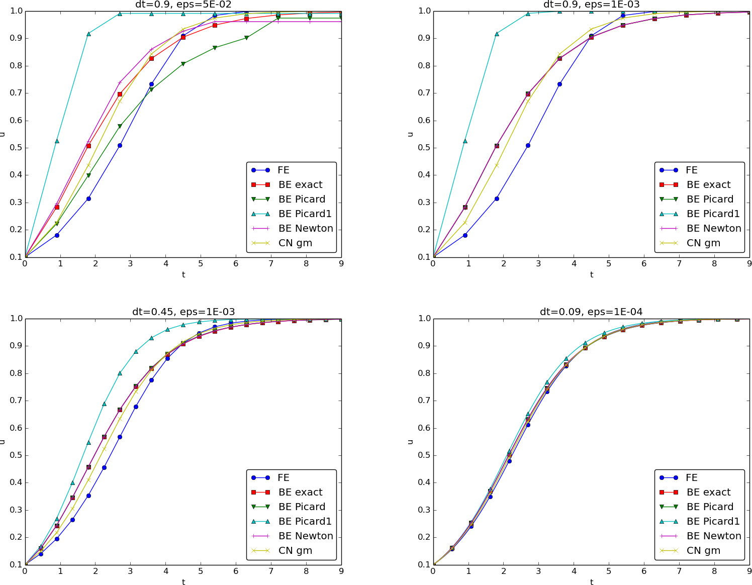
We may run experiments with the model problem (5.1) and the different strategies for dealing with nonlinearities as described above. For a quite coarse time resolution, \(\Delta t=0.9\), use of a tolerance \(\epsilon_r=0.1\) in the stopping criterion introduces an iteration error, especially in the Picard iterations, that is visibly much larger than the time discretization error due to a large \(\Delta t\). This is illustrated by comparing the upper two plots in Figure Figure 5.1. The one to the right has a stricter tolerance \(\epsilon = 10^{-3}\), which causes all the curves corresponding to Picard and Newton iteration to be on top of each other (and no changes can be visually observed by reducing \(\epsilon_r\) further). The reason why Newton’s method does much better than Picard iteration in the upper left plot is that Newton’s method with one step comes far below the \(\epsilon_r\) tolerance, while the Picard iteration needs on average 7 iterations to bring the residual down to \(\epsilon_r=10^{-1}\), which gives insufficient accuracy in the solution of the nonlinear equation. It is obvious that the Picard1 method gives significant errors in addition to the time discretization unless the time step is as small as in the lower right plot.
The BE exact curve corresponds to using the exact solution of the quadratic equation at each time level, so this curve is only affected by the Backward Euler time discretization. The CN gm curve corresponds to the theoretically more accurate Crank-Nicolson discretization, combined with a geometric mean for linearization. This curve appears more accurate, especially if we take the plot in the lower right with a small \(\Delta t\) and an appropriately small \(\epsilon_r\) value as the exact curve.
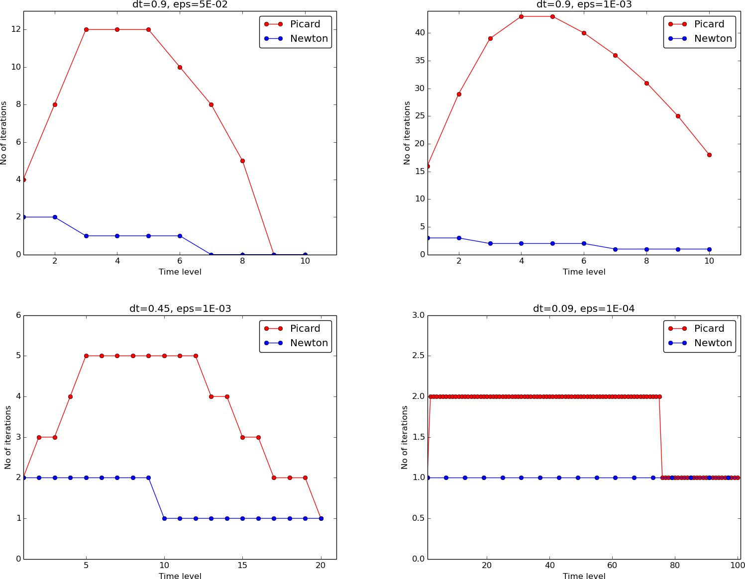
When it comes to the need for iterations, Figure Figure 5.2 displays the number of iterations required at each time level for Newton’s method and Picard iteration. The smaller \(\Delta t\) is, the better starting value we have for the iteration, and the faster the convergence is. With \(\Delta t = 0.9\) Picard iteration requires on average 32 iterations per time step, but this number is dramatically reduced as \(\Delta t\) is reduced.
However, introducing relaxation and a parameter \(\omega=0.8\) immediately reduces the average of 32 to 7, indicating that for the large \(\Delta t=0.9\), Picard iteration takes too long steps. An approximately optimal value for \(\omega\) in this case is 0.5, which results in an average of only 2 iterations! An even more dramatic impact of \(\omega\) appears when \(\Delta t = 1\): Picard iteration does not convergence in 1000 iterations, but \(\omega=0.5\) again brings the average number of iterations down to 2.
Remark. The simple Crank-Nicolson method with a geometric mean for the quadratic nonlinearity gives visually more accurate solutions than the Backward Euler discretization. Even with a tolerance of \(\epsilon_r=10^{-3}\), all the methods for treating the nonlinearities in the Backward Euler discretization give graphs that cannot be distinguished. So for accuracy in this problem, the time discretization is much more crucial than \(\epsilon_r\). Ideally, one should estimate the error in the time discretization, as the solution progresses, and set \(\epsilon_r\) accordingly.
5.11 Generalization to a general nonlinear ODE
Let us see how the various methods in the previous sections can be applied to the more generic model \[ u^{\prime} = f(u, t), \tag{5.10}\] where \(f\) is a nonlinear function of \(u\).
5.11.1 Explicit time discretization
Explicit ODE methods like the Forward Euler scheme, Runge-Kutta methods and Adams-Bashforth methods all evaluate \(f\) at time levels where \(u\) is already computed, so nonlinearities in \(f\) do not pose any difficulties.
5.11.2 Backward Euler discretization
Approximating \(u^{\prime}\) by a backward difference leads to a Backward Euler scheme, which can be written as \[ F(u^n) = u^{n} - \Delta t\, f(u^n, t_n) - u^{n-1}=0, \] or alternatively \[ F(u) = u - \Delta t\, f(u, t_n) - u^{(1)} = 0\tp \] A simple Picard iteration, not knowing anything about the nonlinear structure of \(f\), must approximate \(f(u,t_n)\) by \(f(u^{-},t_n)\): \[ \hat F(u) = u - \Delta t\, f(u^{-},t_n) - u^{(1)}\tp \] The iteration starts with \(u^{-}=u^{(1)}\) and proceeds with repeating \[ u^* = \Delta t\, f(u^{-},t_n) + u^{(1)},\quad u = \omega u^* + (1-\omega)u^{-}, \quad u^{-}\ \leftarrow\ u, \] until a stopping criterion is fulfilled.
Evaluating \(f\) for a known \(u^{-}\) is referred to as explicit treatment of \(f\), while if \(f(u,t)\) has some structure, say \(f(u,t) = u^3\), parts of \(f\) can involve the unknown \(u\), as in the manual linearization \((u^{-})^2u\), and then the treatment of \(f\) is “more implicit” and “less explicit”. This terminology is inspired by time discretization of \(u^{\prime}=f(u,t)\), where evaluating \(f\) for known \(u\) values gives explicit schemes, while treating \(f\) or parts of \(f\) implicitly, makes \(f\) contribute to the unknown terms in the equation at the new time level.
Explicit treatment of \(f\) usually means stricter conditions on \(\Delta t\) to achieve stability of time discretization schemes. The same applies to iteration techniques for nonlinear algebraic equations: the “less” we linearize \(f\) (i.e., the more we keep of \(u\) in the original formula), the faster the convergence may be.
We may say that \(f(u,t)=u^3\) is treated explicitly if we evaluate \(f\) as \((u^{-})^3\), partially implicit if we linearize as \((u^{-})^2u\) and fully implicit if we represent \(f\) by \(u^3\). (Of course, the fully implicit representation will require further linearization, but with \(f(u,t)=u^2\) a fully implicit treatment is possible if the resulting quadratic equation is solved with a formula.)
For the ODE \(u^{\prime}=-u^3\) with \(f(u,t)=-u^3\) and coarse time resolution \(\Delta t = 0.4\), Picard iteration with \((u^{-})^2u\) requires 8 iterations with \(\epsilon_r = 10^{-3}\) for the first time step, while \((u^{-})^3\) leads to 22 iterations. After about 10 time steps both approaches are down to about 2 iterations per time step, but this example shows a potential of treating \(f\) more implicitly.
A trick to treat \(f\) implicitly in Picard iteration is to evaluate it as \(f(u^{-},t)u/u^{-}\). For a polynomial \(f\), \(f(u,t)=u^m\), this corresponds to \((u^{-})^{m}u/u^{-}=(u^{-})^{m-1}u\). Sometimes this more implicit treatment has no effect, as with \(f(u,t)=\exp(-u)\) and \(f(u,t)=\ln (1+u)\), but with \(f(u,t)=\sin(2(u+1))\), the \(f(u^{-},t)u/u^{-}\) trick leads to 7, 9, and 11 iterations during the first three steps, while \(f(u^{-},t)\) demands 17, 21, and 20 iterations. (Experiments can be done with the code ODE_Picard_tricks.py.)
Newton’s method applied to a Backward Euler discretization of \(u^{\prime}=f(u,t)\) requires computation of the derivative \[ F^{\prime}(u) = 1 - \Delta t\frac{\partial f}{\partial u}(u,t_n)\tp \] Starting with the solution at the previous time level, \(u^{-}=u^{(1)}\), we can just use the standard formula \[ u = u^{-} - \omega \frac{F(u^{-})}{F^{\prime}(u^{-})} = u^{-} - \omega \frac{u^{-} - \Delta t\, f(u^{-}, t_n) - u^{(1)}}{1 - \Delta t \frac{\partial}{\partial u}f(u^{-},t_n)} \tp \tag{5.11}\]
5.11.3 Crank-Nicolson discretization
The standard Crank-Nicolson scheme with arithmetic mean approximation of \(f\) takes the form \[ \frac{u^{n+1} - u^n}{\Delta t} = \half(f(u^{n+1}, t_{n+1}) + f(u^n, t_n))\tp \] We can write the scheme as a nonlinear algebraic equation \[ F(u) = u - u^{(1)} - \Delta t{\half}f(u,t_{n+1}) - \Delta t{\half}f(u^{(1)},t_{n}) = 0\tp \tag{5.12}\] A Picard iteration scheme must in general employ the linearization \[ \hat F(u) = u - u^{(1)} - \Delta t{\half}f(u^{-},t_{n+1}) - \Delta t{\half}f(u^{(1)},t_{n}), \] while Newton’s method can apply the general formula (5.11) with \(F(u)\) given in (5.12) and \[ F^{\prime}(u)= 1 - \half\Delta t\frac{\partial f}{\partial u}(u,t_{n+1})\tp \]
5.12 Systems of ODEs
We may write a system of ODEs
\[\begin{align*} \frac{d}{dt}u_0(t) &= f_0(u_0(t),u_1(t),\ldots,u_N(t),t),\\ \frac{d}{dt}u_1(t) &= f_1(u_0(t),u_1(t),\ldots,u_N(t),t),\\ &\vdots\\ \frac{d}{dt}u_m(t) &= f_m(u_0(t),u_1(t),\ldots,u_N(t),t), \end{align*}\] as \[ u^{\prime} = f(u,t),\quad u(0)=U_0, \] if we interpret \(u\) as a vector \(u=(u_0(t),u_1(t),\ldots,u_N(t))\) and \(f\) as a vector function with components \((f_0(u,t),f_1(u,t),\ldots,f_N(u,t))\).
Most solution methods for scalar ODEs, including the Forward and Backward Euler schemes and the Crank-Nicolson method, generalize in a straightforward way to systems of ODEs simply by using vector arithmetics instead of scalar arithmetics, which corresponds to applying the scalar scheme to each component of the system. For example, here is a backward difference scheme applied to each component,
\[\begin{align*} \frac{u_0^n- u_0^{n-1}}{\Delta t} &= f_0(u^n,t_n),\\ \frac{u_1^n- u_1^{n-1}}{\Delta t} &= f_1(u^n,t_n),\\ &\vdots\\ \frac{u_N^n- u_N^{n-1}}{\Delta t} &= f_N(u^n,t_n), \end{align*}\] which can be written more compactly in vector form as \[ \frac{u^n- u^{n-1}}{\Delta t} = f(u^n,t_n)\tp \] This is a system of algebraic equations, \[ u^n - \Delta t\,f(u^n,t_n) - u^{n-1}=0, \] or written out
\[\begin{align*} u_0^n - \Delta t\, f_0(u^n,t_n) - u_0^{n-1} &= 0,\\ &\vdots\\ u_N^n - \Delta t\, f_N(u^n,t_n) - u_N^{n-1} &= 0\tp \end{align*}\]
5.12.1 Example
We shall address the \(2\times 2\) ODE system for oscillations of a pendulum subject to gravity and air drag. The system can be written as
\[\begin{align} \dot\omega &= -\sin\theta -\beta \omega |\omega|,\\ \dot\theta &= \omega, \end{align}\] where \(\beta\) is a dimensionless parameter (this is the scaled, dimensionless version of the original, physical model). The unknown components of the system are the angle \(\theta(t)\) and the angular velocity \(\omega(t)\). We introduce \(u_0=\omega\) and \(u_1=\theta\), which leads to
\[\begin{align*} u_0^{\prime} = f_0(u,t) &= -\sin u_1 - \beta u_0|u_0|,\\ u_1^{\prime} = f_1(u,t) &= u_0\tp \end{align*}\] A Crank-Nicolson scheme reads
\[\begin{align} \frac{u_0^{n+1}-u_0^{n}}{\Delta t} &= -\sin u_1^{n+\frac{1}{2}} - \beta u_0^{n+\frac{1}{2}}|u_0^{n+\frac{1}{2}}|\nonumber\\ & \approx -\sin\left(\frac{1}{2}(u_1^{n+1} + u_1n)\right) - \beta\frac{1}{4} (u_0^{n+1} + u_0^n)|u_0^{n+1}+u_0^n|,\\ \frac{u_1^{n+1}-u_1^n}{\Delta t} &= u_0^{n+\frac{1}{2}}\approx \frac{1}{2} (u_0^{n+1}+u_0^n)\tp \end{align}\] This is a coupled system of two nonlinear algebraic equations in two unknowns \(u_0^{n+1}\) and \(u_1^{n+1}\).
Using the notation \(u_0\) and \(u_1\) for the unknowns \(u_0^{n+1}\) and \(u_1^{n+1}\) in this system, writing \(u_0^{(1)}\) and \(u_1^{(1)}\) for the previous values \(u_0^n\) and \(u_1^n\), multiplying by \(\Delta t\) and moving the terms to the left-hand sides, gives
\[ u_0 - u_0^{(1)} + \Delta t\,\sin\left(\frac{1}{2}(u_1 + u_1^{(1)})\right) + \frac{1}{4}\Delta t\beta (u_0 + u_0^{(1)})|u_0 + u_0^{(1)}| =0, \tag{5.13}\] \[ u_1 - u_1^{(1)} -\frac{1}{2}\Delta t(u_0 + u_0^{(1)}) =0\tp \tag{5.14}\] Obviously, we have a need for solving systems of nonlinear algebraic equations, which is the topic of the next section.
5.13 Systems of nonlinear algebraic equations
Implicit time discretization methods for a system of ODEs, or a PDE, lead to systems of nonlinear algebraic equations, written compactly as \[ F(u) = 0, \] where \(u\) is a vector of unknowns \(u=(u_0,\ldots,u_N)\), and \(F\) is a vector function: \(F=(F_0,\ldots,F_N)\). The system at the end of Section Section 5.12 fits this notation with \(N=1\), \(F_0(u)\) given by the left-hand side of (5.13), while \(F_1(u)\) is the left-hand side of (5.14).
Sometimes the equation system has a special structure because of the underlying problem, e.g., \[ A(u)u = b(u), \] with \(A(u)\) as an \((N+1)\times (N+1)\) matrix function of \(u\) and \(b\) as a vector function: \(b=(b_0,\ldots,b_N)\).
We shall next explain how Picard iteration and Newton’s method can be applied to systems like \(F(u)=0\) and \(A(u)u=b(u)\). The exposition has a focus on ideas and practical computations. More theoretical considerations, including quite general results on convergence properties of these methods, can be found in Kelley (Kelley 1995).
5.14 Picard iteration
We cannot apply Picard iteration to nonlinear equations unless there is some special structure. For the commonly arising case \(A(u)u=b(u)\) we can linearize the product \(A(u)u\) to \(A(u^{-})u\) and \(b(u)\) as \(b(u^{-})\). That is, we use the most previously computed approximation in \(A\) and \(b\) to arrive at a linear system for \(u\): \[ A(u^{-})u = b(u^{-})\tp \] A relaxed iteration takes the form \[ A(u^{-})u^* = b(u^{-}),\quad u = \omega u^* + (1-\omega)u^{-}\tp \] In other words, we solve a system of nonlinear algebraic equations as a sequence of linear systems.
Given \(A(u)u=b(u)\) and an initial guess \(u^{-}\), iterate until convergence:
- solve \(A(u^{-})u^* = b(u^{-})\) with respect to \(u^*\)
- \(u = \omega u^* + (1-\omega) u^{-}\)
- \(u^{-}\ \leftarrow\ u\)
“Until convergence” means that the iteration is stopped when the change in the unknown, \(||u - u^{-}||\), or the residual \(||A(u)u-b||\), is sufficiently small, see Section Section 5.16 for more details.
5.15 Newton’s method
The natural starting point for Newton’s method is the general nonlinear vector equation \(F(u)=0\). As for a scalar equation, the idea is to approximate \(F\) around a known value \(u^{-}\) by a linear function \(\hat F\), calculated from the first two terms of a Taylor expansion of \(F\). In the multi-variate case these two terms become \[ F(u^{-}) + J(u^{-}) \cdot (u - u^{-}), \] where \(J\) is the Jacobian of \(F\), defined by \[ J_{i,j} = \frac{\partial F_i}{\partial u_j}\tp \] So, the original nonlinear system is approximated by \[ \hat F(u) = F(u^{-}) + J(u^{-}) \cdot (u - u^{-})=0, \] which is linear in \(u\) and can be solved in a two-step procedure: first solve \(J\delta u = -F(u^{-})\) with respect to the vector \(\delta u\) and then update \(u = u^{-} + \delta u\). A relaxation parameter can easily be incorporated: \[ u = \omega(u^{-} +\delta u) + (1-\omega)u^{-} = u^{-} + \omega\delta u\tp \]
Given \(F(u)=0\) and an initial guess \(u^{-}\), iterate until convergence:
- solve \(J\delta u = -F(u^{-})\) with respect to \(\delta u\)
- \(u = u^{-} + \omega\delta u\)
- \(u^{-}\ \leftarrow\ u\)
For the special system with structure \(A(u)u=b(u)\), \[ F_i = \sum_k A_{i,k}(u)u_k - b_i(u), \] one gets \[ J_{i,j} = \sum_k \frac{\partial A_{i,k}}{\partial u_j}u_k + A_{i,j} - \frac{\partial b_i}{\partial u_j}\tp \] We realize that the Jacobian needed in Newton’s method consists of \(A(u^{-})\) as in the Picard iteration plus two additional terms arising from the differentiation. Using the notation \(A^{\prime}(u)\) for \(\partial A/\partial u\) (a quantity with three indices: \(\partial A_{i,k}/\partial u_j\)), and \(b^{\prime}(u)\) for \(\partial b/\partial u\) (a quantity with two indices: \(\partial b_i/\partial u_j\)), we can write the linear system to be solved as \[ (A + A^{\prime}u + b^{\prime})\delta u = -Au + b, \] or \[ (A(u^{-}) + A^{\prime}(u^{-})u^{-} + b^{\prime}(u^{-}))\delta u = -A(u^{-})u^{-} + b(u^{-})\tp \] Rearranging the terms demonstrates the difference from the system solved in each Picard iteration: \[ \underbrace{A(u^{-})(u^{-}+\delta u) - b(u^{-})}_{\text{Picard system}} +\, \gamma (A^{\prime}(u^{-})u^{-} + b^{\prime}(u^{-}))\delta u = 0\tp \] Here we have inserted a parameter \(\gamma\) such that \(\gamma=0\) gives the Picard system and \(\gamma=1\) gives the Newton system. Such a parameter can be handy in software to easily switch between the methods.
Given \(A(u)\), \(b(u)\), and an initial guess \(u^{-}\), iterate until convergence:
- solve \((A + \gamma(A^{\prime}(u^{-})u^{-} + b^{\prime}(u^{-})))\delta u = -A(u^{-})u^{-} + b(u^{-})\) with respect to \(\delta u\)
- \(u = u^{-} + \omega\delta u\)
- \(u^{-}\ \leftarrow\ u\)
\(\gamma =1\) gives a Newton method while \(\gamma =0\) corresponds to Picard iteration.
5.16 Stopping criteria
Let \(||\cdot||\) be the standard Euclidean vector norm. Four termination criteria are much in use:
- Absolute change in solution: \(||u - u^{-}||\leq \epsilon_u\)
- Relative change in solution: \(||u - u^{-}||\leq \epsilon_u ||u_0||\), where \(u_0\) denotes the start value of \(u^{-}\) in the iteration
- Absolute residual: \(||F(u)|| \leq \epsilon_r\)
- Relative residual: \(||F(u)|| \leq \epsilon_r ||F(u_0)||\)
To prevent divergent iterations to run forever, one terminates the iterations when the current number of iterations \(k\) exceeds a maximum value \(k_{\max}\).
The relative criteria are most used since they are not sensitive to the characteristic size of \(u\). Nevertheless, the relative criteria can be misleading when the initial start value for the iteration is very close to the solution, since an unnecessary reduction in the error measure is enforced. In such cases the absolute criteria work better. It is common to combine the absolute and relative measures of the size of the residual, as in \[ ||F(u)|| \leq \epsilon_{rr} ||F(u_0)|| + \epsilon_{ra}, \] where \(\epsilon_{rr}\) is the tolerance in the relative criterion and \(\epsilon_{ra}\) is the tolerance in the absolute criterion. With a very good initial guess for the iteration (typically the solution of a differential equation at the previous time level), the term \(||F(u_0)||\) is small and \(\epsilon_{ra}\) is the dominating tolerance. Otherwise, \(\epsilon_{rr} ||F(u_0)||\) and the relative criterion dominates.
With the change in solution as criterion we can formulate a combined absolute and relative measure of the change in the solution: \[ ||\delta u|| \leq \epsilon_{ur} ||u_0|| + \epsilon_{ua}, \] The ultimate termination criterion, combining the residual and the change in solution with a test on the maximum number of iterations, can be expressed as \[ ||F(u)|| \leq \epsilon_{rr} ||F(u_0)|| + \epsilon_{ra} \quad\text{or}\quad ||\delta u|| \leq \epsilon_{ur} ||u_0|| + \epsilon_{ua} \quad\text{or}\quad k>k_{\max}\tp \] ## Example: A nonlinear ODE model from epidemiology {#sec-nonlin-systems-alg-SI}
A very simple model for the spreading of a disease, such as a flu, takes the form of a \(2\times 2\) ODE system
\[\begin{align} S^{\prime} &= -\beta SI,\\ I^{\prime} &= \beta SI - \nu I, \end{align}\] where \(S(t)\) is the number of people who can get ill (susceptibles) and \(I(t)\) is the number of people who are ill (infected). The constants \(\beta >0\) and \(\nu >0\) must be given along with initial conditions \(S(0)\) and \(I(0)\).
5.16.1 Implicit time discretization
A Crank-Nicolson scheme leads to a \(2\times 2\) system of nonlinear algebraic equations in the unknowns \(S^{n+1}\) and \(I^{n+1}\):
\[\begin{align} \frac{S^{n+1}-S^n}{\Delta t} &= -\beta [SI]^{n+\half} \approx -\frac{\beta}{2}(S^nI^n + S^{n+1}I^{n+1}),\\ \frac{I^{n+1}-I^n}{\Delta t} &= \beta [SI]^{n+\half} - \nu I^{n+\half} \approx \frac{\beta}{2}(S^nI^n + S^{n+1}I^{n+1}) - \frac{\nu}{2}(I^n + I^{n+1})\tp \end{align}\] Introducing \(S\) for \(S^{n+1}\), \(S^{(1)}\) for \(S^n\), \(I\) for \(I^{n+1}\) and \(I^{(1)}\) for \(I^n\), we can rewrite the system as
\[ F_S(S,I) = S - S^{(1)} + \half\Delta t\beta(S^{(1)}I^{(1)} + SI) = 0, \tag{5.15}\] \[ F_I(S,I) = I - I^{(1)} - \half\Delta t\beta(S^{(1)}I^{(1)} + SI) + \half\Delta t\nu(I^{(1)} + I) =0\tp \tag{5.16}\]
5.16.2 A Picard iteration
We assume that we have approximations \(S^{-}\) and \(I^{-}\) to \(S\) and \(I\), respectively. A way of linearizing the only nonlinear term \(SI\) is to write \(I^{-}S\) in the \(F_S=0\) equation and \(S^{-}I\) in the \(F_I=0\) equation, which also decouples the equations. Solving the resulting linear equations with respect to the unknowns \(S\) and \(I\) gives
\[\begin{align*} S &= \frac{S^{(1)} - \half\Delta t\beta S^{(1)}I^{(1)}} {1 + \half\Delta t\beta I^{-}}, \\ I &= \frac{I^{(1)} + \half\Delta t\beta S^{(1)}I^{(1)} - \half\Delta t\nu I^{(1)}} {1 - \half\Delta t\beta S^{-} + \half\Delta t \nu}\tp \end{align*}\] Before a new iteration, we must update \(S^{-}\ \leftarrow\ S\) and \(I^{-}\ \leftarrow\ I\).
5.16.3 Newton’s method
The nonlinear system (5.15)-(5.16) can be written as \(F(u)=0\) with \(F=(F_S,F_I)\) and \(u=(S,I)\). The Jacobian becomes \[ J = \left(\begin{array}{cc} \frac{\partial}{\partial S} F_S & \frac{\partial}{\partial I}F_S\\ \frac{\partial}{\partial S} F_I & \frac{\partial}{\partial I}F_I \end{array}\right) = \left(\begin{array}{cc} 1 + \half\Delta t\beta I & \half\Delta t\beta S\\ + \half\Delta t\beta I & 1 - \half\Delta t\beta S + \half\Delta t\nu \end{array}\right) \tp \] The Newton system \(J(u^{-})\delta u = -F(u^{-})\) to be solved in each iteration is then
\[\begin{align*} & \left(\begin{array}{cc} 1 + \half\Delta t\beta I^{-} & \half\Delta t\beta S^{-}\\ - \half\Delta t\beta I^{-} & 1 - \half\Delta t\beta S^{-} + \half\Delta t\nu \end{array}\right) \left(\begin{array}{c} \delta S\\ \delta I \end{array}\right) =\\ & \qquad\qquad \left(\begin{array}{c} S^{-} - S^{(1)} + \half\Delta t\beta(S^{(1)}I^{(1)} + S^{-}I^{-})\\ I^{-} - I^{(1)} - \half\Delta t\beta(S^{(1)}I^{(1)} + S^{-}I^{-}) + \half\Delta t\nu(I^{(1)} + I^{-}) \end{array}\right) \end{align*}\]
Remark. For this particular system of ODEs, explicit time integration methods work very well. Even a Forward Euler scheme is fine, but (as also experienced more generally) the 4-th order Runge-Kutta method is an excellent balance between high accuracy, high efficiency, and simplicity.
5.17 Nonlinear diffusion model
The attention is now turned to nonlinear partial differential equations (PDEs) and application of the techniques explained above for ODEs. The model problem is a nonlinear diffusion equation for \(u(\x,t)\):
\[\begin{alignat}{2} \frac{\partial u}{\partial t} &= \nabla\cdot (\dfc(u)\nabla u) + f(u),\quad &\x\in\Omega,\ t\in (0,T], \\ -\dfc(u)\frac{\partial u}{\partial n} &= g,\quad &\x\in\partial\Omega_N,\ t\in (0,T], \\ u &= u_0,\quad &\x\in\partial\Omega_D,\ t\in (0,T]\tp \end{alignat}\]In the present section, our aim is to discretize this problem in time and then present techniques for linearizing the time-discrete PDE problem “at the PDE level” such that we transform the nonlinear stationary PDE problem at each time level into a sequence of linear PDE problems, which can be solved using any method for linear PDEs. This strategy avoids the solution of systems of nonlinear algebraic equations. In Section Section 5.22 we shall take the opposite (and more common) approach: discretize the nonlinear problem in time and space first, and then solve the resulting nonlinear algebraic equations at each time level by the methods of Section Section 5.13. Very often, the two approaches are mathematically identical, so there is no preference from a computational efficiency point of view. The details of the ideas sketched above will hopefully become clear through the forthcoming examples.
5.18 Explicit time integration
The nonlinearities in the PDE are trivial to deal with if we choose an explicit time integration method for the nonlinear diffusion equation, such as the Forward Euler method: \[ [D_t^+ u = \nabla\cdot (\dfc(u)\nabla u) + f(u)]^n, \] or written out, \[ \frac{u^{n+1} - u^n}{\Delta t} = \nabla\cdot (\dfc(u^n)\nabla u^n) + f(u^n), \] which is a linear equation in the unknown \(u^{n+1}\) with solution \[ u^{n+1} = u^n + \Delta t\nabla\cdot (\dfc(u^n)\nabla u^n) + \Delta t f(u^n)\tp \] The disadvantage with this discretization is the strict stability criterion \(\Delta t \leq h^2/(6\max\alpha)\) for the case \(f=0\) and a standard 2nd-order finite difference discretization in 3D space with mesh cell sizes \(h=\Delta x=\Delta y=\Delta z\).
5.19 Backward Euler scheme and Picard iteration
A Backward Euler scheme for the nonlinear diffusion equation reads \[ [D_t^- u = \nabla\cdot (\dfc(u)\nabla u) + f(u)]^n\tp \] Written out, \[ \frac{u^{n} - u^{n-1}}{\Delta t} = \nabla\cdot (\dfc(u^n)\nabla u^n) + f(u^n)\tp \tag{5.17}\] This is a nonlinear PDE for the unknown function \(u^n(\x)\). Such a PDE can be viewed as a time-independent PDE where \(u^{n-1}(\x)\) is a known function.
We introduce a Picard iteration with \(k\) as iteration counter. A typical linearization of the \(\nabla\cdot(\dfc(u^n)\nabla u^n)\) term in iteration \(k+1\) is to use the previously computed \(u^{n,k}\) approximation in the diffusion coefficient: \(\dfc(u^{n,k})\). The nonlinear source term is treated similarly: \(f(u^{n,k})\). The unknown function \(u^{n,k+1}\) then fulfills the linear PDE \[ \frac{u^{n,k+1} - u^{n-1}}{\Delta t} = \nabla\cdot (\dfc(u^{n,k}) \nabla u^{n,k+1}) + f(u^{n,k})\tp \tag{5.18}\] The initial guess for the Picard iteration at this time level can be taken as the solution at the previous time level: \(u^{n,0}=u^{n-1}\).
We can alternatively apply the implementation-friendly notation where \(u\) corresponds to the unknown we want to solve for, i.e., \(u^{n,k+1}\) above, and \(u^{-}\) is the most recently computed value, \(u^{n,k}\) above. Moreover, \(u^{(1)}\) denotes the unknown function at the previous time level, \(u^{n-1}\) above. The PDE to be solved in a Picard iteration then looks like \[ \frac{u - u^{(1)}}{\Delta t} = \nabla\cdot (\dfc(u^{-}) \nabla u) + f(u^{-})\tp \tag{5.19}\] At the beginning of the iteration we start with the value from the previous time level: \(u^{-}=u^{(1)}\), and after each iteration, \(u^{-}\) is updated to \(u\).
The previous derivations of the numerical scheme for time discretizations of PDEs have, strictly speaking, a somewhat sloppy notation, but it is much used and convenient to read. A more precise notation must distinguish clearly between the exact solution of the PDE problem, here denoted \(u_{\text{e}}(\x,t)\), and the exact solution of the spatial problem, arising after time discretization at each time level, where (5.17) is an example. The latter is here represented as \(u^n(\x)\) and is an approximation to \(u_{\text{e}}(\x,t_n)\). Then we have another approximation \(u^{n,k}(\x)\) to \(u^n(\x)\) when solving the nonlinear PDE problem for \(u^n\) by iteration methods, as in (5.18).
In our notation, \(u\) is a synonym for \(u^{n,k+1}\) and \(u^{(1)}\) is a synonym for \(u^{n-1}\), inspired by what are natural variable names in a code. We will usually state the PDE problem in terms of \(u\) and quickly redefine the symbol \(u\) to mean the numerical approximation, while \(u_{\text{e}}\) is not explicitly introduced unless we need to talk about the exact solution and the approximate solution at the same time.
5.20 Backward Euler scheme and Newton’s method
At time level \(n\), we have to solve the stationary PDE (5.17). In the previous section, we saw how this can be done with Picard iterations. Another alternative is to apply the idea of Newton’s method in a clever way. Normally, Newton’s method is defined for systems of algebraic equations, but the idea of the method can be applied at the PDE level too.
5.20.1 Linearization via Taylor expansions
Let \(u^{n,k}\) be an approximation to the unknown \(u^n\). We seek a better approximation on the form \[ u^{n} = u^{n,k} + \delta u\tp \tag{5.20}\] The idea is to insert (5.20) in (5.17), Taylor expand the nonlinearities and keep only the terms that are linear in \(\delta u\) (which makes (5.20) an approximation for \(u^{n}\)). Then we can solve a linear PDE for the correction \(\delta u\) and use (5.20) to find a new approximation \[ u^{n,k+1}=u^{n,k}+\delta u \] to \(u^{n}\). Repeating this procedure gives a sequence \(u^{n,k+1}\), \(k=0,1,\ldots\) that hopefully converges to the goal \(u^n\).
Let us carry out all the mathematical details for the nonlinear diffusion PDE discretized by the Backward Euler method. Inserting (5.20) in (5.17) gives \[ \frac{u^{n,k} +\delta u - u^{n-1}}{\Delta t} = \nabla\cdot (\dfc(u^{n,k} + \delta u)\nabla (u^{n,k}+\delta u)) + f(u^{n,k}+\delta u)\tp \tag{5.21}\] We can Taylor expand \(\dfc(u^{n,k} + \delta u)\) and \(f(u^{n,k}+\delta u)\):
\[\begin{align*} \dfc(u^{n,k} + \delta u) & = \dfc(u^{n,k}) + \frac{d\dfc}{du}(u^{n,k}) \delta u + \Oof{\delta u^2}\approx \dfc(u^{n,k}) + \dfc^{\prime}(u^{n,k})\delta u,\\ f(u^{n,k}+\delta u) &= f(u^{n,k}) + \frac{df}{du}(u^{n,k})\delta u + \Oof{\delta u^2}\approx f(u^{n,k}) + f^{\prime}(u^{n,k})\delta u\tp \end{align*}\] Inserting the linear approximations of \(\dfc\) and \(f\) in (5.21) results in
\[ \begin{split} \frac{u^{n,k} +\delta u - u^{n-1}}{\Delta t} &= \nabla\cdot (\dfc(u^{n,k})\nabla u^{n,k}) + f(u^{n,k}) + \\ &\qquad \nabla\cdot (\dfc(u^{n,k})\nabla \delta u) + \nabla\cdot (\dfc^{\prime}(u^{n,k})\delta u\nabla u^{n,k}) + \\ &\qquad \nabla\cdot (\dfc^{\prime}(u^{n,k})\delta u\nabla \delta u) + f^{\prime}(u^{n,k})\delta u\tp \end{split} \tag{5.22}\] The term \(\dfc^{\prime}(u^{n,k})\delta u\nabla \delta u\) is of order \(\delta u^2\) and therefore omitted since we expect the correction \(\delta u\) to be small (\(\delta u \gg \delta u^2\)). Reorganizing the equation gives a PDE for \(\delta u\) that we can write in short form as \[ \delta F(\delta u; u^{n,k}) = -F(u^{n,k}), \] where
\[ F(u^{n,k}) = \frac{u^{n,k} - u^{n-1}}{\Delta t} - \nabla\cdot (\dfc(u^{n,k})\nabla u^{n,k}) + f(u^{n,k}), \] \[ \begin{split} \delta F(\delta u; u^{n,k}) &= - \frac{1}{\Delta t}\delta u + \nabla\cdot (\dfc(u^{n,k})\nabla \delta u) + \\ &\quad \nabla\cdot (\dfc^{\prime}(u^{n,k})\delta u\nabla u^{n,k}) + f^{\prime}(u^{n,k})\delta u\tp \end{split} \tag{5.23}\] Note that \(\delta F\) is a linear function of \(\delta u\), and \(F\) contains only terms that are known, such that the PDE for \(\delta u\) is indeed linear.
The notational form \(\delta F = -F\) resembles the Newton system \(J\delta u =-F\) for systems of algebraic equations, with \(\delta F\) as \(J\delta u\). The unknown vector in a linear system of algebraic equations enters the system as a linear operator in terms of a matrix-vector product (\(J\delta u\)), while at the PDE level we have a linear differential operator instead (\(\delta F\)).
5.20.2 Similarity with Picard iteration
We can rewrite the PDE for \(\delta u\) in a slightly different way too if we define \(u^{n,k} + \delta u\) as \(u^{n,k+1}\).
\[\begin{align} & \frac{u^{n,k+1} - u^{n-1}}{\Delta t} = \nabla\cdot (\dfc(u^{n,k})\nabla u^{n,k+1}) + f(u^{n,k})\nonumber\\ &\qquad + \nabla\cdot (\dfc^{\prime}(u^{n,k})\delta u\nabla u^{n,k}) + f^{\prime}(u^{n,k})\delta u\tp \end{align}\] Note that the first line is the same PDE as arises in the Picard iteration, while the remaining terms arise from the differentiations that are an inherent ingredient in Newton’s method.
5.20.3 Implementation
For coding we want to introduce \(u\) for \(u^n\), \(u^{-}\) for \(u^{n,k}\) and \(u^{(1)}\) for \(u^{n-1}\). The formulas for \(F\) and \(\delta F\) are then more clearly written as
\[ F(u^{-}) = \frac{u^{-} - u^{(1)}}{\Delta t} - \nabla\cdot (\dfc(u^{-})\nabla u^{-}) + f(u^{-}), \] \[ \begin{split} \delta F(\delta u; u^{-}) &= - \frac{1}{\Delta t}\delta u + \nabla\cdot (\dfc(u^{-})\nabla \delta u) + \\ &\quad \nabla\cdot (\dfc^{\prime}(u^{-})\delta u\nabla u^{-}) + f^{\prime}(u^{-})\delta u\tp \end{split} \tag{5.24}\] The form that orders the PDE as the Picard iteration terms plus the Newton method’s derivative terms becomes
\[\begin{align} & \frac{u - u^{(1)}}{\Delta t} = \nabla\cdot (\dfc(u^{-})\nabla u) + f(u^{-}) + \nonumber\\ &\qquad \gamma(\nabla\cdot (\dfc^{\prime}(u^{-})(u - u^{-})\nabla u^{-}) + f^{\prime}(u^{-})(u - u^{-}))\tp \end{align}\] The Picard and full Newton versions correspond to \(\gamma=0\) and \(\gamma=1\), respectively.
5.20.4 Derivation with alternative notation
Some may prefer to derive the linearized PDE for \(\delta u\) using the more compact notation. We start with inserting \(u^n=u^{-}+\delta u\) to get \[ \frac{u^{-} +\delta u - u^{n-1}}{\Delta t} = \nabla\cdot (\dfc(u^{-} + \delta u)\nabla (u^{-}+\delta u)) + f(u^{-}+\delta u)\tp \] Taylor expanding,
\[\begin{align*} \dfc(u^{-} + \delta u) & \approx \dfc(u^{-}) + \dfc^{\prime}(u^{-})\delta u,\\ f(u^{-}+\delta u) & \approx f(u^{-}) + f^{\prime}(u^{-})\delta u, \end{align*}\] and inserting these expressions gives a less cluttered PDE for \(\delta u\):
\[\begin{align*} \frac{u^{-} +\delta u - u^{n-1}}{\Delta t} &= \nabla\cdot (\dfc(u^{-})\nabla u^{-}) + f(u^{-}) + \\ &\qquad \nabla\cdot (\dfc(u^{-})\nabla \delta u) + \nabla\cdot (\dfc^{\prime}(u^{-})\delta u\nabla u^{-}) + \\ &\qquad \nabla\cdot (\dfc^{\prime}(u^{-})\delta u\nabla \delta u) + f^{\prime}(u^{-})\delta u\tp \end{align*}\]
5.21 Crank-Nicolson discretization
A Crank-Nicolson discretization of the nonlinear diffusion equation applies a centered difference at \(t_{n+\frac{1}{2}}\): \[ [D_t u = \nabla\cdot (\dfc(u)\nabla u) + f(u)]^{n+\frac{1}{2}}\tp \] The standard technique is to apply an arithmetic average for quantities defined between two mesh points, e.g., \[ u^{n+\frac{1}{2}}\approx \frac{1}{2}(u^n + u^{n+1})\tp \] However, with nonlinear terms we have many choices of formulating an arithmetic mean:
\[\begin{align} [f(u)]^{n+\frac{1}{2}} &\approx f(\frac{1}{2}(u^n + u^{n+1})) = [f(\overline{u}^t)]^{n+\frac{1}{2}},\\ [f(u)]^{n+\frac{1}{2}} &\approx \frac{1}{2}(f(u^n) + f(u^{n+1})) =[\overline{f(u)}^t]^{n+\frac{1}{2}},\\ [\dfc(u)\nabla u]^{n+\frac{1}{2}} &\approx \dfc(\frac{1}{2}(u^n + u^{n+1}))\nabla (\frac{1}{2}(u^n + u^{n+1})) = [\dfc(\overline{u}^t)\nabla \overline{u}^t]^{n+\frac{1}{2}},\\ [\dfc(u)\nabla u]^{n+\frac{1}{2}} &\approx \frac{1}{2}(\dfc(u^n) + \dfc(u^{n+1}))\nabla (\frac{1}{2}(u^n + u^{n+1})) = [\overline{\dfc(u)}^t\nabla\overline{u}^t]^{n+\frac{1}{2}},\\ [\dfc(u)\nabla u]^{n+\frac{1}{2}} &\approx \frac{1}{2}(\dfc(u^n)\nabla u^n + \dfc(u^{n+1})\nabla u^{n+1}) = [\overline{\dfc(u)\nabla u}^t]^{n+\frac{1}{2}}\tp \end{align}\]
A big question is whether there are significant differences in accuracy between taking the products of arithmetic means or taking the arithmetic mean of products. Exercise Section 5.42 investigates this question, and the answer is that the approximation is \(\Oof{\Delta t^2}\) in both cases.
5.22 Discretization in space and Newton’s method
Section Section 5.17 presented methods for linearizing time-discrete PDEs directly prior to discretization in space. We can alternatively carry out the discretization in space of the time-discrete nonlinear PDE problem and get a system of nonlinear algebraic equations, which can be solved by Picard iteration or Newton’s method as presented in Section Section 5.13. This latter approach will now be described in detail.
We shall work with the 1D problem \[ -(\dfc(u)u^{\prime})^{\prime} + au = f(u),\quad x\in (0,L), \quad \dfc(u(0))u^{\prime}(0) = C,\ u(L)=D \tp \tag{5.25}\]
The problem (5.25) arises from the stationary limit of a diffusion equation, \[ \frac{\partial u}{\partial t} = \frac{\partial}{\partial x}\left( \alpha(u)\frac{\partial u}{\partial x}\right) - au + f(u), \tag{5.26}\] as \(t\rightarrow\infty\) and \(\partial u/\partial t\rightarrow 0\). Alternatively, the problem (5.25) arises at each time level from implicit time discretization of (5.26). For example, a Backward Euler scheme for (5.26) leads to \[ \frac{u^{n}-u^{n-1}}{\Delta t} = \frac{d}{dx}\left( \alpha(u^n)\frac{du^n}{dx}\right) - au^n + f(u^n)\tp \tag{5.27}\] Introducing \(u(x)\) for \(u^n(x)\), \(u^{(1)}\) for \(u^{n-1}\), and defining \(f(u)\) in (5.25) to be \(f(u)\) in (5.27) plus \(u^{n-1}/\Delta t\), gives (5.25) with \(a=1/\Delta t\).
5.23 Finite difference discretization
The nonlinearity in the differential equation (5.25) poses no more difficulty than a variable coefficient, as in the term \((\dfc(x)u^{\prime})^{\prime}\). We can therefore use a standard finite difference approach when discretizing the Laplace term with a variable coefficient: \[ [-D_x\dfc D_x u +au = f]_i\tp \] Writing this out for a uniform mesh with points \(x_i=i\Delta x\), \(i=0,\ldots,N_x\), leads to
\[ -\frac{1}{\Delta x^2} \left(\dfc_{i+\half}(u_{i+1}-u_i) - \dfc_{i-\half}(u_{i}-u_{i-1})\right) + au_i = f(u_i)\tp \tag{5.28}\] This equation is valid at all the mesh points \(i=0,1,\ldots,N_x-1\). At \(i=N_x\) we have the Dirichlet condition \(u_i=0\). The only difference from the case with \((\dfc(x)u^{\prime})^{\prime}\) and \(f(x)\) is that now \(\dfc\) and \(f\) are functions of \(u\) and not only of \(x\): \((\dfc(u(x))u^{\prime})^{\prime}\) and \(f(u(x))\).
The quantity \(\dfc_{i+\half}\), evaluated between two mesh points, needs a comment. Since \(\dfc\) depends on \(u\) and \(u\) is only known at the mesh points, we need to express \(\dfc_{i+\half}\) in terms of \(u_i\) and \(u_{i+1}\). For this purpose we use an arithmetic mean, although a harmonic mean is also common in this context if \(\dfc\) features large jumps. There are two choices of arithmetic means:
\[ \dfc_{i+\half} \approx \dfc(\half(u_i + u_{i+1}) = [\dfc(\overline{u}^x)]^{i+\half}, \] \[ \dfc_{i+\half} \approx \half(\dfc(u_i) + \dfc(u_{i+1})) = [\overline{\dfc(u)}^x]^{i+\half} \tag{5.29}\] Equation (5.28) with the latter approximation then looks like
\[ \begin{split} &-\frac{1}{2\Delta x^2} \left((\dfc(u_i)+\dfc(u_{i+1}))(u_{i+1}-u_i) - (\dfc(u_{i-1})+\dfc(u_{i}))(u_{i}-u_{i-1})\right)\\ &\qquad\qquad + au_i = f(u_i), \end{split} \tag{5.30}\] or written more compactly, \[ [-D_x\overline{\dfc}^x D_x u +au = f]_i\tp \] At mesh point \(i=0\) we have the boundary condition \(\dfc(u)u^{\prime}=C\), which is discretized by \[ [\dfc(u)D_{2x}u = C]_0, \] meaning \[ \dfc(u_0)\frac{u_{1} - u_{-1}}{2\Delta x} = C\tp \tag{5.31}\] The fictitious value \(u_{-1}\) can be eliminated with the aid of (5.30) for \(i=0\). Formally, (5.30) should be solved with respect to \(u_{i-1}\) and that value (for \(i=0\)) should be inserted in (5.31), but it is algebraically much easier to do it the other way around. Alternatively, one can use a ghost cell \([-\Delta x,0]\) and update the \(u_{-1}\) value in the ghost cell according to (5.31) after every Picard or Newton iteration. Such an approach means that we use a known \(u_{-1}\) value in (5.30) from the previous iteration.
5.24 Solution of algebraic equations
5.24.1 The structure of the equation system
The nonlinear algebraic equations (5.30) are of the form \(A(u)u = b(u)\) with
\[\begin{align*} A_{i,i} &= \frac{1}{2\Delta x^2}(\dfc(u_{i-1}) + 2\dfc(u_{i}) \dfc(u_{i+1})) + a,\\ A_{i,i-1} &= -\frac{1}{2\Delta x^2}(\dfc(u_{i-1}) + \dfc(u_{i})),\\ A_{i,i+1} &= -\frac{1}{2\Delta x^2}(\dfc(u_{i}) + \dfc(u_{i+1})),\\ b_i &= f(u_i)\tp \end{align*}\] The matrix \(A(u)\) is tridiagonal: \(A_{i,j}=0\) for \(j > i+1\) and \(j < i-1\).
The above expressions are valid for internal mesh points \(1\leq i\leq N_x-1\). For \(i=0\) we need to express \(u_{i-1}=u_{-1}\) in terms of \(u_1\) using (5.31): \[ u_{-1} = u_1 -\frac{2\Delta x}{\dfc(u_0)}C\tp \tag{5.32}\] This value must be inserted in \(A_{0,0}\). The expression for \(A_{i,i+1}\) applies for \(i=0\), and \(A_{i,i-1}\) does not enter the system when \(i=0\).
Regarding the last equation, its form depends on whether we include the Dirichlet condition \(u(L)=D\), meaning \(u_{N_x}=D\), in the nonlinear algebraic equation system or not. Suppose we choose \((u_0,u_1,\ldots,u_{N_x-1})\) as unknowns, later referred to as systems without Dirichlet conditions. The last equation corresponds to \(i=N_x-1\). It involves the boundary value \(u_{N_x}\), which is substituted by \(D\). If the unknown vector includes the boundary value, \((u_0,u_1,\ldots,u_{N_x})\), later referred to as system including Dirichlet conditions, the equation for \(i=N_x-1\) just involves the unknown \(u_{N_x}\), and the final equation becomes \(u_{N_x}=D\), corresponding to \(A_{i,i}=1\) and \(b_i=D\) for \(i=N_x\).
5.24.2 Picard iteration
The obvious Picard iteration scheme is to use previously computed values of \(u_i\) in \(A(u)\) and \(b(u)\), as described more in detail in Section Section 5.13. With the notation \(u^{-}\) for the most recently computed value of \(u\), we have the system \(F(u)\approx \hat F(u) = A(u^{-})u - b(u^{-})\), with \(F=(F_0,F_1,\ldots,F_m)\), \(u=(u_0,u_1,\ldots,u_m)\). The index \(m\) is \(N_x\) if the system includes the Dirichlet condition as a separate equation and \(N_x-1\) otherwise. The matrix \(A(u^{-})\) is tridiagonal, so the solution procedure is to fill a tridiagonal matrix data structure and the right-hand side vector with the right numbers and call a Gaussian elimination routine for tridiagonal linear systems.
5.24.3 Mesh with two cells
It helps on the understanding of the details to write out all the mathematics in a specific case with a small mesh, say just two cells (\(N_x=2\)). We use \(u^{-}_i\) for the \(i\)-th component in \(u^{-}\).
The starting point is the basic expressions for the nonlinear equations at mesh point \(i=0\) and \(i=1\):
\[ A_{0,-1}u_{-1} + A_{0,0}u_0 + A_{0,1}u_1 = b_0, \tag{5.33}\] \[ A_{1,0}u_{0} + A_{1,1}u_1 + A_{1,2}u_2 = b_1\tp \tag{5.34}\] Equation (5.33) written out reads
\[\begin{align*} \frac{1}{2\Delta x^2}(& -(\dfc(u_{-1}) + \dfc(u_{0}))u_{-1}\, +\\ & (\dfc(u_{-1}) + 2\dfc(u_{0}) + \dfc(u_{1}))u_0\, -\\ & (\dfc(u_{0}) + \dfc(u_{1})))u_1 + au_0 =f(u_0)\tp \end{align*}\] We must then replace \(u_{-1}\) by (5.32). With Picard iteration we get
\[\begin{align*} \frac{1}{2\Delta x^2}(& -(\dfc(u^-_{-1}) + 2\dfc(u^-_{0}) + \dfc(u^-_{1}))u_1\, +\\ &(\dfc(u^-_{-1}) + 2\dfc(u^-_{0}) + \dfc(u^-_{1}))u_0 + au_0\\ &=f(u^-_0) - \frac{1}{\dfc(u^-_0)\Delta x}(\dfc(u^-_{-1}) + \dfc(u^-_{0}))C, \end{align*}\] where \[ u^-_{-1} = u_1^- -\frac{2\Delta x}{\dfc(u^-_0)}C\tp \] Equation (5.34) contains the unknown \(u_2\) for which we have a Dirichlet condition. In case we omit the condition as a separate equation, (5.34) with Picard iteration becomes
\[\begin{align*} \frac{1}{2\Delta x^2}(&-(\dfc(u^-_{0}) + \dfc(u^-_{1}))u_{0}\, + \\ &(\dfc(u^-_{0}) + 2\dfc(u^-_{1}) + \dfc(u^-_{2}))u_1\, -\\ &(\dfc(u^-_{1}) + \dfc(u^-_{2})))u_2 + au_1 =f(u^-_1)\tp \end{align*}\] We must now move the \(u_2\) term to the right-hand side and replace all occurrences of \(u_2\) by \(D\):
\[\begin{align*} \frac{1}{2\Delta x^2}(&-(\dfc(u^-_{0}) + \dfc(u^-_{1}))u_{0}\, +\\ & (\dfc(u^-_{0}) + 2\dfc(u^-_{1}) + \dfc(D)))u_1 + au_1\\ &=f(u^-_1) + \frac{1}{2\Delta x^2}(\dfc(u^-_{1}) + \dfc(D))D\tp \end{align*}\]
The two equations can be written as a \(2\times 2\) system: \[ \left(\begin{array}{cc} B_{0,0}& B_{0,1}\\ B_{1,0} & B_{1,1} \end{array}\right) \left(\begin{array}{c} u_0\\ u_1 \end{array}\right) = \left(\begin{array}{c} d_0\\ d_1 \end{array}\right), \] where
\[\begin{align} B_{0,0} &=\frac{1}{2\Delta x^2}(\dfc(u^-_{-1}) + 2\dfc(u^-_{0}) + \dfc(u^-_{1})) + a,\\ B_{0,1} &= -\frac{1}{2\Delta x^2}(\dfc(u^-_{-1}) + 2\dfc(u^-_{0}) + \dfc(u^-_{1})),\\ B_{1,0} &= -\frac{1}{2\Delta x^2}(\dfc(u^-_{0}) + \dfc(u^-_{1})),\\ B_{1,1} &= \frac{1}{2\Delta x^2}(\dfc(u^-_{0}) + 2\dfc(u^-_{1}) + \dfc(D)) + a,\\ d_0 &= f(u^-_0) - \frac{1}{\dfc(u^-_0)\Delta x}(\dfc(u^-_{-1}) + \dfc(u^-_{0}))C,\\ d_1 &= f(u^-_1) + \frac{1}{2\Delta x^2}(\dfc(u^-_{1}) + \dfc(D))D\tp \end{align}\]
The system with the Dirichlet condition becomes \[ \left(\begin{array}{ccc} B_{0,0}& B_{0,1} & 0\\ B_{1,0} & B_{1,1} & B_{1,2}\\ 0 & 0 & 1 \end{array}\right) \left(\begin{array}{c} u_0\\ u_1\\ u_2 \end{array}\right) = \left(\begin{array}{c} d_0\\ d_1\\ D \end{array}\right), \] with
\[\begin{align} B_{1,1} &= \frac{1}{2\Delta x^2}(\dfc(u^-_{0}) + 2\dfc(u^-_{1}) + \dfc(u_2)) + a,\\ B_{1,2} &= - \frac{1}{2\Delta x^2}(\dfc(u^-_{1}) + \dfc(u_2))),\\ d_1 &= f(u^-_1)\tp \end{align}\] Other entries are as in the \(2\times 2\) system.
5.24.4 Newton’s method
Using Newton’s method requires deriving the Jacobian. Here it means that we need to differentiate \(F(u)=A(u)u - b(u)\) with respect to the unknown parameters \(u_0,u_1,\ldots,u_m\) (\(m=N_x\) or \(m=N_x-1\), depending on whether the Dirichlet condition is included in the nonlinear system \(F(u)=0\) or not). Nonlinear equation number \(i\) has the structure \[ F_i = A_{i,i-1}(u_{i-1},u_i)u_{i-1} + A_{i,i}(u_{i-1},u_i,u_{i+1})u_i + A_{i,i+1}(u_i, u_{i+1})u_{i+1} - b_i(u_i)\tp \] Computing the Jacobian requires careful differentiation. For example,
\[\begin{align*} \frac{\partial}{\partial u_i}(A_{i,i}(u_{i-1},u_i,u_{i+1})u_i) &= \frac{\partial A_{i,i}}{\partial u_i}u_i + A_{i,i} \frac{\partial u_i}{\partial u_i}\\ &= \frac{\partial}{\partial u_i}( \frac{1}{2\Delta x^2}(\dfc(u_{i-1}) + 2\dfc(u_{i}) +\dfc(u_{i+1})) + a)u_i +\\ &\quad\frac{1}{2\Delta x^2}(\dfc(u_{i-1}) + 2\dfc(u_{i}) +\dfc(u_{i+1})) + a\\ &= \frac{1}{2\Delta x^2}(2\dfc^\prime (u_i)u_i +\dfc(u_{i-1}) + 2\dfc(u_{i}) +\dfc(u_{i+1})) + a\tp \end{align*}\] The complete Jacobian becomes
\[\begin{align*} J_{i,i} &= \frac{\partial F_i}{\partial u_i} = \frac{\partial A_{i,i-1}}{\partial u_i}u_{i-1} + \frac{\partial A_{i,i}}{\partial u_i}u_i + A_{i,i} + \frac{\partial A_{i,i+1}}{\partial u_i}u_{i+1} - \frac{\partial b_i}{\partial u_{i}}\\ &= \frac{1}{2\Delta x^2}( -\dfc^{\prime}(u_i)u_{i-1} +2\dfc^{\prime}(u_i)u_{i} +\dfc(u_{i-1}) + 2\dfc(u_i) + \dfc(u_{i+1})) +\\ &\quad a -\frac{1}{2\Delta x^2}\dfc^{\prime}(u_{i})u_{i+1} - b^{\prime}(u_i),\\ J_{i,i-1} &= \frac{\partial F_i}{\partial u_{i-1}} = \frac{\partial A_{i,i-1}}{\partial u_{i-1}}u_{i-1} + A_{i-1,i} + \frac{\partial A_{i,i}}{\partial u_{i-1}}u_i - \frac{\partial b_i}{\partial u_{i-1}}\\ &= \frac{1}{2\Delta x^2}( -\dfc^{\prime}(u_{i-1})u_{i-1} - (\dfc(u_{i-1}) + \dfc(u_i)) + \dfc^{\prime}(u_{i-1})u_i),\\ J_{i,i+1} &= \frac{\partial A_{i,i+1}}{\partial u_{i-1}}u_{i+1} + A_{i+1,i} + \frac{\partial A_{i,i}}{\partial u_{i+1}}u_i - \frac{\partial b_i}{\partial u_{i+1}}\\ &=\frac{1}{2\Delta x^2}( -\dfc^{\prime}(u_{i+1})u_{i+1} - (\dfc(u_{i}) + \dfc(u_{i+1})) + \dfc^{\prime}(u_{i+1})u_i) \end{align*}\] The explicit expression for nonlinear equation number \(i\), \(F_i(u_0,u_1,\ldots)\), arises from moving the \(f(u_i)\) term in (5.30) to the left-hand side:
\[ \begin{split} F_i &= -\frac{1}{2\Delta x^2} \left((\dfc(u_i)+\dfc(u_{i+1}))(u_{i+1}-u_i) - (\dfc(u_{i-1})+\dfc(u_{i}))(u_{i}-u_{i-1})\right)\\ &\qquad\qquad + au_i - f(u_i) = 0\tp \end{split} \tag{5.35}\]
At the boundary point \(i=0\), \(u_{-1}\) must be replaced using the formula (5.32). When the Dirichlet condition at \(i=N_x\) is not a part of the equation system, the last equation \(F_m=0\) for \(m=N_x-1\) involves the quantity \(u_{N_x-1}\) which must be replaced by \(D\). If \(u_{N_x}\) is treated as an unknown in the system, the last equation \(F_m=0\) has \(m=N_x\) and reads \[ F_{N_x}(u_0,\ldots,u_{N_x}) = u_{N_x} - D = 0\tp \] Similar replacement of \(u_{-1}\) and \(u_{N_x}\) must be done in the Jacobian for the first and last row. When \(u_{N_x}\) is included as an unknown, the last row in the Jacobian must help implement the condition \(\delta u_{N_x}=0\), since we assume that \(u\) contains the right Dirichlet value at the beginning of the iteration (\(u_{N_x}=D\)), and then the Newton update should be zero for \(i=0\), i.e., \(\delta u_{N_x}=0\). This also forces the right-hand side to be \(b_i=0\), \(i=N_x\).
We have seen, and can see from the present example, that the linear system in Newton’s method contains all the terms present in the system that arises in the Picard iteration method. The extra terms in Newton’s method can be multiplied by a factor such that it is easy to program one linear system and set this factor to 0 or 1 to generate the Picard or Newton system.
5.25 Solving Nonlinear PDEs with Devito
Having established the finite difference discretization of nonlinear PDEs, we now implement several solvers using Devito. The symbolic approach allows us to express nonlinear equations and handle the time-lagged coefficients naturally.
5.25.1 Nonlinear Diffusion: The Explicit Scheme
The nonlinear diffusion equation \[ u_t = \nabla \cdot (D(u) \nabla u) \] with solution-dependent diffusivity \(D(u)\) requires special treatment. In 1D, the equation becomes: \[ u_t = \frac{\partial}{\partial x}\left(D(u) \frac{\partial u}{\partial x}\right) \]
For explicit time stepping, we evaluate \(D\) at the previous time level: \[ u^{n+1}_i = u^n_i + \frac{\Delta t}{\Delta x^2} \left[D^n_{i+1/2}(u^n_{i+1} - u^n_i) - D^n_{i-1/2}(u^n_i - u^n_{i-1})\right] \]
where \(D^n_{i+1/2} = \frac{1}{2}(D(u^n_i) + D(u^n_{i+1}))\).
5.25.2 The Devito Implementation
from devito import Grid, TimeFunction, Eq, Operator, Constant
import numpy as np

# Domain and discretization
L = 1.0           # Domain length
Nx = 100          # Grid points
T = 0.1           # Final time
F = 0.4           # Target Fourier number

dx = L / Nx
D_max = 1.0       # Maximum diffusion coefficient
dt = F * dx**2 / D_max  # Time step from stability

# Create Devito grid
grid = Grid(shape=(Nx + 1,), extent=(L,))

# Time-varying field with space_order=2 for halo access
u = TimeFunction(name='u', grid=grid, time_order=1, space_order=2)
5.25.3 Handling the Nonlinear Diffusion Coefficient
For nonlinear diffusion, the diffusivity depends on the solution. Common forms include:
| Type | \(D(u)\) | Application |
|---|---|---|
| Constant | \(D_0\) | Linear heat conduction |
| Linear | \(D_0(1 + \alpha u)\) | Temperature-dependent conductivity |
| Porous medium | \(D_0 m u^{m-1}\) | Flow in porous media |
The src.nonlin module provides several diffusion coefficient functions:
from src.nonlin import (
    constant_diffusion,
    linear_diffusion,
    porous_medium_diffusion,
)

# Constant D(u) = 1.0
D_const = lambda u: constant_diffusion(u, D0=1.0)

# Linear D(u) = 1 + 0.5*u
D_linear = lambda u: linear_diffusion(u, D0=1.0, alpha=0.5)

# Porous medium D(u) = 2*u (m=2)
D_porous = lambda u: porous_medium_diffusion(u, m=2.0, D0=1.0)
5.25.4 Complete Nonlinear Diffusion Solver
The src.nonlin module provides solve_nonlinear_diffusion_explicit:
from src.nonlin import solve_nonlinear_diffusion_explicit
import numpy as np

# Initial condition: smooth bump
def I(x):
    return np.sin(np.pi * x)

result = solve_nonlinear_diffusion_explicit(
    L=1.0,           # Domain length
    Nx=100,          # Grid points
    T=0.1,           # Final time
    F=0.4,           # Fourier number
    I=I,             # Initial condition
    D_func=lambda u: linear_diffusion(u, D0=1.0, alpha=0.5),
)

print(f"Final time: {result.t:.4f}")
print(f"Max solution: {result.u.max():.6f}")
5.25.5 Reaction-Diffusion with Operator Splitting
The reaction-diffusion equation \[ u_t = a u_{xx} + R(u) \] combines diffusion with a nonlinear reaction term. Operator splitting separates these effects:
Lie Splitting (first-order): 1. Solve \(u_t = a u_{xx}\) for time \(\Delta t\) 2. Solve \(u_t = R(u)\) for time \(\Delta t\)
Strang Splitting (second-order): 1. Solve \(u_t = R(u)\) for time \(\Delta t/2\) 2. Solve \(u_t = a u_{xx}\) for time \(\Delta t\) 3. Solve \(u_t = R(u)\) for time \(\Delta t/2\)
5.25.6 Reaction Terms
The module provides common reaction terms:
from src.nonlin import (
    logistic_reaction,
    fisher_reaction,
    allen_cahn_reaction,
)

# Logistic growth: R(u) = r*u*(1 - u/K)
R_logistic = lambda u: logistic_reaction(u, r=1.0, K=1.0)

# Fisher-KPP: R(u) = r*u*(1 - u)
R_fisher = lambda u: fisher_reaction(u, r=1.0)

# Allen-Cahn: R(u) = u - u^3
R_allen_cahn = lambda u: allen_cahn_reaction(u, epsilon=1.0)
5.25.7 Reaction-Diffusion Solver
from src.nonlin import solve_reaction_diffusion_splitting

# Initial condition with small perturbation
def I(x):
    return 0.5 * np.sin(np.pi * x)

# Strang splitting (second-order)
result = solve_reaction_diffusion_splitting(
    L=1.0,
    a=0.1,           # Diffusion coefficient
    Nx=100,
    T=0.5,
    F=0.4,
    I=I,
    R_func=lambda u: fisher_reaction(u, r=1.0),
    splitting="strang",
)
The Strang splitting achieves second-order accuracy in time, while Lie splitting is only first-order. For problems with fast reactions or long simulation times, the higher accuracy of Strang splitting is beneficial.
5.25.8 Burgers’ Equation
The viscous Burgers’ equation \[ u_t + u u_x = \nu u_{xx} \] is a prototype for nonlinear advection with viscous dissipation. The nonlinear term \(u u_x\) can cause shock formation for small \(\nu\).
We use the conservative form \((u^2/2)_x\) with centered differences:
from src.nonlin import solve_burgers_equation

result = solve_burgers_equation(
    L=2.0,           # Domain length
    nu=0.01,         # Viscosity
    Nx=100,          # Grid points
    T=0.5,           # Final time
    C=0.5,           # Target CFL number
)
5.25.9 Stability for Burgers’ Equation
The time step must satisfy both the CFL condition for advection: \[ C = \frac{|u|_{\max} \Delta t}{\Delta x} \le 1 \]
and the diffusion stability condition: \[ F = \frac{\nu \Delta t}{\Delta x^2} \le 0.5 \]
The solver automatically chooses \(\Delta t\) to satisfy both conditions with a safety factor.
5.25.10 The Effect of Viscosity
import matplotlib.pyplot as plt

fig, axes = plt.subplots(1, 2, figsize=(12, 5))

for ax, nu in zip(axes, [0.1, 0.01]):
    result = solve_burgers_equation(
        L=2.0, nu=nu, Nx=100, T=0.5, C=0.3,
        I=lambda x: np.sin(np.pi * x),
        save_history=True,
    )

    for i in range(0, len(result.t_history), len(result.t_history)//5):
        ax.plot(result.x, result.u_history[i],
                label=f't = {result.t_history[i]:.2f}')

    ax.set_xlabel('x')
    ax.set_ylabel('u')
    ax.set_title(f'Burgers, nu = {nu}')
    ax.legend()
Higher viscosity (\(\nu = 0.1\)) smooths the solution, while lower viscosity (\(\nu = 0.01\)) allows steeper gradients to develop.
5.25.11 Picard Iteration for Implicit Schemes
For stiff nonlinear problems, implicit time stepping may be necessary. Picard iteration solves the nonlinear system by repeated linearization:
- Guess \(u^{n+1, (0)} = u^n\)
- For \(k = 0, 1, 2, \ldots\):
- Evaluate \(D^{(k)} = D(u^{n+1, (k)})\)
- Solve the linear system for \(u^{n+1, (k+1)}\)
- Check convergence: \(\|u^{n+1, (k+1)} - u^{n+1, (k)}\| < \epsilon\)
from src.nonlin import solve_nonlinear_diffusion_picard

result = solve_nonlinear_diffusion_picard(
    L=1.0,
    Nx=50,
    T=0.05,
    dt=0.001,        # Can use larger dt than explicit
)
The implicit scheme removes the time step restriction but requires solving a linear system at each iteration.
5.25.12 Summary
Key points for nonlinear PDEs with Devito:
- Nonlinear diffusion: Use explicit scheme with lagged coefficient evaluation and Fourier number \(F \le 0.5\)
- Operator splitting: Separates diffusion and reaction for reaction-diffusion equations; Strang is second-order
- Burgers’ equation: Requires both CFL and diffusion stability conditions; viscosity controls smoothness
- Picard iteration: Enables implicit schemes for stiff problems at the cost of solving linear systems
The src.nonlin module provides: - solve_nonlinear_diffusion_explicit - solve_reaction_diffusion_splitting - solve_burgers_equation - solve_nonlinear_diffusion_picard - Diffusion coefficients: constant_diffusion, linear_diffusion, porous_medium_diffusion - Reaction terms: logistic_reaction, fisher_reaction, allen_cahn_reaction
5.26 2D Burgers Equation with Devito
The Burgers equation is a fundamental nonlinear PDE that combines advection and diffusion. It serves as a prototype for understanding shock formation, numerical stability in nonlinear problems, and provides insight into the Navier-Stokes equations.
5.26.1 The Coupled Burgers Equations
The 2D coupled Burgers equations describe a simplified model of viscous fluid flow:
\[ \frac{\partial u}{\partial t} + u \frac{\partial u}{\partial x} + v \frac{\partial u}{\partial y} = \nu \left(\frac{\partial^2 u}{\partial x^2} + \frac{\partial^2 u}{\partial y^2}\right) \tag{5.36}\]
\[ \frac{\partial v}{\partial t} + u \frac{\partial v}{\partial x} + v \frac{\partial v}{\partial y} = \nu \left(\frac{\partial^2 v}{\partial x^2} + \frac{\partial^2 v}{\partial y^2}\right) \tag{5.37}\]
Here \(u\) and \(v\) are velocity components, and \(\nu\) is the viscosity (kinematic). The left-hand side represents nonlinear advection (transport of the field by itself), while the right-hand side represents viscous diffusion.
5.26.2 Physical Interpretation
The Burgers equation exhibits several important physical phenomena:
| Feature | Description |
|---|---|
| Advection | \(u \partial u/\partial x\) causes wave steepening |
| Diffusion | \(\nu \nabla^2 u\) smooths gradients |
| Shock formation | When advection dominates, discontinuities develop |
| Balance | Viscosity prevents infinite gradients |
The ratio of advection to diffusion is characterized by the Reynolds number: \(\text{Re} = UL/\nu\), where \(U\) is a characteristic velocity and \(L\) is a length scale. High Reynolds numbers (low viscosity) lead to steep gradients or shocks.
5.26.3 Discretization Strategy
The Burgers equation requires careful treatment of the advection terms. Using centered differences for \(u \partial u/\partial x\) leads to instability. Instead, we use upwind differencing for advection:
Advection terms (first-order backward): \[ u \frac{\partial u}{\partial x} \approx u_{i,j}^n \frac{u_{i,j}^n - u_{i-1,j}^n}{\Delta x} \]
Diffusion terms (second-order centered): \[ \frac{\partial^2 u}{\partial x^2} \approx \frac{u_{i+1,j}^n - 2u_{i,j}^n + u_{i-1,j}^n}{\Delta x^2} \]
This mixed discretization uses:
- First-order backward differences (
fd_order=1,side=left) for advection - Second-order centered differences (
.laplace) for diffusion
5.26.4 Implementation with first_derivative
Devito’s first_derivative function allows explicit control over the finite difference order and stencil direction:
This code is included from src/book_snippets/burgers_first_derivative.py and exercised by pytest (see tests/test_book_snippets.py).
from devito import Grid, TimeFunction, first_derivative, left

# Create grid and velocity fields
Nx, Ny = 41, 41
Lx, Ly = 2.0, 2.0

grid = Grid(shape=(Nx, Ny), extent=(Lx, Ly))
x, y = grid.dimensions

u = TimeFunction(name="u", grid=grid, time_order=1, space_order=2)
v = TimeFunction(name="v", grid=grid, time_order=1, space_order=2)

# First-order backward differences for advection
# fd_order=1 gives first-order accuracy
# side=left gives backward difference: (u[x] - u[x-dx]) / dx
u_dx = first_derivative(u, dim=x, side=left, fd_order=1)
u_dy = first_derivative(u, dim=y, side=left, fd_order=1)
v_dx = first_derivative(v, dim=x, side=left, fd_order=1)
v_dy = first_derivative(v, dim=y, side=left, fd_order=1)

# Verify the stencil structure
RESULT = {
    "u_dx": str(u_dx),
    "u_dy": str(u_dy),
}
The key parameters are:
| Parameter | Purpose | Example |
|---|---|---|
dim |
Differentiation dimension | x or y |
side |
Stencil direction | left (backward) |
fd_order |
Finite difference order | 1 for first-order |
5.26.5 Building the Burgers Equations and Boundary Conditions
With the explicit derivatives defined, we write the equations and boundary conditions. The subdomain=grid.interior ensures the stencil is only applied away from boundaries, where we set Dirichlet conditions separately:
This code is included from src/book_snippets/burgers_equations_bc.py and exercised by pytest (see tests/test_book_snippets.py).
from devito import (
    Constant,
    Eq,
    Grid,
    Operator,
    TimeFunction,
    first_derivative,
    left,
    solve,
)

# Create grid and velocity fields
Nx, Ny = 41, 41
Lx, Ly = 2.0, 2.0

grid = Grid(shape=(Nx, Ny), extent=(Lx, Ly))
x, y = grid.dimensions

u = TimeFunction(name="u", grid=grid, time_order=1, space_order=2)
v = TimeFunction(name="v", grid=grid, time_order=1, space_order=2)

# First-order backward differences for advection
u_dx = first_derivative(u, dim=x, side=left, fd_order=1)
u_dy = first_derivative(u, dim=y, side=left, fd_order=1)
v_dx = first_derivative(v, dim=x, side=left, fd_order=1)
v_dy = first_derivative(v, dim=y, side=left, fd_order=1)

# Viscosity as symbolic constant
nu = Constant(name="nu")

# Burgers equations with backward advection and centered diffusion
# u_t + u*u_x + v*u_y = nu * laplace(u)
eq_u = Eq(u.dt + u * u_dx + v * u_dy, nu * u.laplace, subdomain=grid.interior)
eq_v = Eq(v.dt + u * v_dx + v * v_dy, nu * v.laplace, subdomain=grid.interior)

# Solve for the update expressions
stencil_u = solve(eq_u, u.forward)
stencil_v = solve(eq_v, v.forward)

update_u = Eq(u.forward, stencil_u)
update_v = Eq(v.forward, stencil_v)

# Boundary conditions
t = grid.stepping_dim
bc_value = 1.0  # Boundary condition value

# u boundary conditions
bc_u = [Eq(u[t + 1, 0, y], bc_value)]  # left
bc_u += [Eq(u[t + 1, Nx - 1, y], bc_value)]  # right
bc_u += [Eq(u[t + 1, x, 0], bc_value)]  # bottom
bc_u += [Eq(u[t + 1, x, Ny - 1], bc_value)]  # top

# v boundary conditions (similar)
bc_v = [Eq(v[t + 1, 0, y], bc_value)]  # left
bc_v += [Eq(v[t + 1, Nx - 1, y], bc_value)]  # right
bc_v += [Eq(v[t + 1, x, 0], bc_value)]  # bottom
bc_v += [Eq(v[t + 1, x, Ny - 1], bc_value)]  # top

# Create operator with updates and boundary conditions
op = Operator([update_u, update_v] + bc_u + bc_v)

RESULT = {
    "num_equations": len([update_u, update_v] + bc_u + bc_v),
    "grid_shape": grid.shape,
}
5.26.6 Alternative: VectorTimeFunction Approach
For coupled vector equations like Burgers, Devito’s VectorTimeFunction provides a more compact notation. The velocity field is represented as a single vector \(\mathbf{U} = (u, v)\):
\[ \frac{\partial \mathbf{U}}{\partial t} + (\nabla \mathbf{U}) \cdot \mathbf{U} = \nu \nabla^2 \mathbf{U} \]
from devito import VectorTimeFunction, grad

# Create vector velocity field
U = VectorTimeFunction(name='U', grid=grid, space_order=2)

# U[0] is u-component, U[1] is v-component
# Initialize components
U[0].data[0, :, :] = u_initial
U[1].data[0, :, :] = v_initial

# Vector form of Burgers equation
# U_forward = U - dt * (grad(U)*U - nu * laplace(U))
s = grid.time_dim.spacing  # dt symbol
update_U = Eq(U.forward, U - s * (grad(U)*U - nu*U.laplace),
              subdomain=grid.interior)

# The grad(U)*U term represents advection:
# [u*u_x + v*u_y]
# [u*v_x + v*v_y]
This approach is mathematically elegant and maps directly to the vector notation used in fluid dynamics.
5.26.7 Using the Solver
The src.nonlin.burgers_devito module provides ready-to-use solvers:
from src.nonlin.burgers_devito import (
    solve_burgers_2d,
    solve_burgers_2d_vector,
    init_hat,
)

# Solve with scalar TimeFunction approach
result = solve_burgers_2d(
    Lx=2.0, Ly=2.0,   # Domain size
    nu=0.01,           # Viscosity
    Nx=41, Ny=41,      # Grid points
    T=0.5,             # Final time
    sigma=0.0009,      # Stability parameter
)

print(f"Final time: {result.t}")
print(f"u range: [{result.u.min():.3f}, {result.u.max():.3f}]")
print(f"v range: [{result.v.min():.3f}, {result.v.max():.3f}]")
5.26.8 Stability Considerations
The explicit scheme requires satisfying both advection and diffusion stability conditions:
CFL condition for advection: \[ C = \frac{|u|_{\max} \Delta t}{\Delta x} \leq 1 \]
Fourier condition for diffusion (2D): \[ F = \frac{\nu \Delta t}{\Delta x^2} \leq 0.25 \]
The solver uses: \[ \Delta t = \sigma \frac{\Delta x \cdot \Delta y}{\nu} \] where \(\sigma\) is a small stability parameter (default 0.0009).
5.26.9 Visualizing Shock Formation
The evolution shows how the initially sharp “hat” profile evolves:
import matplotlib.pyplot as plt
from src.nonlin.burgers_devito import solve_burgers_2d

# Low viscosity case - steeper gradients
result = solve_burgers_2d(
    Lx=2.0, Ly=2.0,
    nu=0.01,
    Nx=41, Ny=41,
    T=0.5,
    save_history=True,
    save_every=100,
)

fig, axes = plt.subplots(1, len(result.t_history), figsize=(15, 4))
for i, (t, u) in enumerate(zip(result.t_history, result.u_history)):
    axes[i].contourf(result.x, result.y, u.T, levels=20)
    axes[i].set_title(f't = {t:.3f}')
    axes[i].set_xlabel('x')
    axes[i].set_ylabel('y')
plt.tight_layout()
5.26.10 Effect of Viscosity
Comparing low and high viscosity reveals the balance between advection and diffusion:
from src.nonlin.burgers_devito import solve_burgers_2d
import matplotlib.pyplot as plt

fig, axes = plt.subplots(1, 2, figsize=(12, 5))

for ax, nu, title in zip(axes, [0.1, 0.01], ['High viscosity', 'Low viscosity']):
    result = solve_burgers_2d(
        Lx=2.0, Ly=2.0,
        nu=nu,
        Nx=41, Ny=41,
        T=0.5,
    )
    c = ax.contourf(result.x, result.y, result.u.T, levels=20)
    ax.set_title(f'{title} (nu={nu})')
    ax.set_xlabel('x')
    ax.set_ylabel('y')
    plt.colorbar(c, ax=ax)
With high viscosity (\(\nu = 0.1\)), diffusion dominates and the solution smooths rapidly. With low viscosity (\(\nu = 0.01\)), advection dominates, the “hat” moves and steepens, and gradients remain sharper.
5.26.11 Comparison: Scalar vs Vector Implementation
Both implementations solve the same equations but offer different trade-offs:
| Aspect | Scalar (solve_burgers_2d) |
Vector (solve_burgers_2d_vector) |
|---|---|---|
| Derivatives | Explicit first_derivative() |
Implicit via grad(U)*U |
| Control | Full control over stencils | Uses default differentiation |
| Code length | More verbose | More compact |
| Debugging | Easier to inspect | More opaque |
For production use where precise control over numerical schemes is needed, the scalar approach with explicit first_derivative() is preferred. The vector approach is useful for rapid prototyping and when the default schemes are acceptable.
5.26.12 Summary
Key points for solving Burgers equation with Devito:
- Mixed discretization: Use first-order upwind for advection, second-order centered for diffusion
- first_derivative(): Enables explicit control of stencil order and direction via
fd_orderandsideparameters - VectorTimeFunction: Alternative approach using
grad(U)*Ufor more compact code - Stability: Must satisfy both CFL and Fourier conditions
- Viscosity: Controls the balance between sharp gradients (shocks) and smooth solutions
The module src.nonlin.burgers_devito provides:
solve_burgers_2d: Scalar implementation with explicit derivativessolve_burgers_2d_vector: Vector implementation usingVectorTimeFunctioninit_hat: Classic hat-function initial conditionsinusoidal_initial_condition: Smooth sinusoidal initial datagaussian_initial_condition: Gaussian pulse initial data
The fundamental ideas in the derivation of \(F_i\) and \(J_{i,j}\) in the 1D model problem are easily generalized to multi-dimensional problems. Nevertheless, the expressions involved are slightly different, with derivatives in \(x\) replaced by \(\nabla\), so we present some examples below in detail.
5.27 Finite difference discretization
A typical diffusion equation \[ u_t = \nabla\cdot(\dfc(u)\nabla u) + f(u), \] can be discretized by (e.g.) a Backward Euler scheme, which in 2D can be written \[ [D_t^- u = D_x\overline{\dfc(u)}^xD_x u + D_y\overline{\dfc(u)}^yD_y u + f(u)]_{i,j}^n\tp \] We do not dive into the details of handling boundary conditions now. Dirichlet and Neumann conditions are handled as in corresponding linear, variable-coefficient diffusion problems.
Writing the scheme out, putting the unknown values on the left-hand side and known values on the right-hand side, and introducing \(\Delta x=\Delta y=h\) to save some writing, one gets
\[\begin{align*} u^n_{i,j} &- \frac{\Delta t}{h^2}( \half(\dfc(u_{i,j}^n) + \dfc(u_{i+1,j}^n))(u_{i+1,j}^n-u_{i,j}^n)\\ &\quad - \half(\dfc(u_{i-1,j}^n) + \dfc(u_{i,j}^n))(u_{i,j}^n-u_{i-1,j}^n) \\ &\quad + \half(\dfc(u_{i,j}^n) + \dfc(u_{i,j+1}^n))(u_{i,j+1}^n-u_{i,j}^n)\\ &\quad - \half(\dfc(u_{i,j-1}^n) + \dfc(u_{i,j}^n))(u_{i,j}^n-u_{i-1,j-1}^n)) - \Delta tf(u_{i,j}^n) = u^{n-1}_{i,j} \end{align*}\] This defines a nonlinear algebraic system on the form \(A(u)u=b(u)\).
5.27.1 Picard iteration
The most recently computed values \(u^{-}\) of \(u^n\) can be used in \(\dfc\) and \(f\) for a Picard iteration, or equivalently, we solve \(A(u^{-})u=b(u^{-})\). The result is a linear system of the same type as arising from \(u_t = \nabla\cdot (\dfc(\x)\nabla u) + f(\x,t)\).
The Picard iteration scheme can also be expressed in operator notation: \[ [D_t^- u = D_x\overline{\dfc(u^{-})}^xD_x u + D_y\overline{\dfc(u^{-})}^yD_y u + f(u^{-})]_{i,j}^n\tp \] ### Newton’s method
As always, Newton’s method is technically more involved than Picard iteration. We first define the nonlinear algebraic equations to be solved, drop the superscript \(n\) (use \(u\) for \(u^n\)), and introduce \(u^{(1)}\) for \(u^{n-1}\):
\[\begin{align*} F_{i,j} &= u_{i,j} - \frac{\Delta t}{h^2}(\\ &\qquad \half(\dfc(u_{i,j}) + \dfc(u_{i+1,j}))(u_{i+1,j}-u_{i,j}) -\\ &\qquad \half(\dfc(u_{i-1,j}) + \dfc(u_{i,j}))(u_{i,j}-u_{i-1,j}) + \\ &\qquad \half(\dfc(u_{i,j}) + \dfc(u_{i,j+1}))(u_{i,j+1}-u_{i,j}) -\\ &\qquad \half(\dfc(u_{i,j-1}) + \dfc(u_{i,j}))(u_{i,j}-u_{i-1,j-1})) - \Delta t\, f(u_{i,j}) - u^{(1)}_{i,j} = 0\tp \end{align*}\] It is convenient to work with two indices \(i\) and \(j\) in 2D finite difference discretizations, but it complicates the derivation of the Jacobian, which then gets four indices. (Make sure you really understand the 1D version of this problem as treated in Section Section 5.23.) The left-hand expression of an equation \(F_{i,j}=0\) is to be differentiated with respect to each of the unknowns \(u_{r,s}\) (recall that this is short notation for \(u_{r,s}^n\)), \(r\in\Ix\), \(s\in\Iy\): \[ J_{i,j,r,s} = \frac{\partial F_{i,j}}{\partial u_{r,s}}\tp \] The Newton system to be solved in each iteration can be written as \[ \sum_{r\in\Ix}\sum_{s\in\Iy}J_{i,j,r,s}\delta u_{r,s} = -F_{i,j}, \quad i\in\Ix,\ j\in\Iy\tp \] Given \(i\) and \(j\), only a few \(r\) and \(s\) indices give nonzero contribution to the Jacobian since \(F_{i,j}\) contains \(u_{i\pm 1,j}\), \(u_{i,j\pm 1}\), and \(u_{i,j}\). This means that \(J_{i,j,r,s}\) has nonzero contributions only if \(r=i\pm 1\), \(s=j\pm 1\), as well as \(r=i\) and \(s=j\). The corresponding terms in \(J_{i,j,r,s}\) are \(J_{i,j,i-1,j}\), \(J_{i,j,i+1,j}\), \(J_{i,j,i,j-1}\), \(J_{i,j,i,j+1}\) and \(J_{i,j,i,j}\). Therefore, the left-hand side of the Newton system, \(\sum_r\sum_s J_{i,j,r,s}\delta u_{r,s}\) collapses to
\[\begin{align*} J_{i,j,r,s}\delta u_{r,s} = J_{i,j,i,j}\delta u_{i,j} & + J_{i,j,i-1,j}\delta u_{i-1,j} + J_{i,j,i+1,j}\delta u_{i+1,j} + J_{i,j,i,j-1}\delta u_{i,j-1}\\ & + J_{i,j,i,j+1}\delta u_{i,j+1} \end{align*}\] The specific derivatives become
\[\begin{align*} J_{i,j,i-1,j} &= \frac{\partial F_{i,j}}{\partial u_{i-1,j}}\\ &= \frac{\Delta t}{h^2}(\dfc^{\prime}(u_{i-1,j})(u_{i,j}-u_{i-1,j}) - \dfc(u_{i-1,j})(-1)),\\ J_{i,j,i+1,j} &= \frac{\partial F_{i,j}}{\partial u_{i+1,j}}\\ &= \frac{\Delta t}{h^2}(-\dfc^{\prime}(u_{i+1,j})(u_{i+1,j}-u_{i,j}) - \dfc(u_{i-1,j})),\\ J_{i,j,i,j-1} &= \frac{\partial F_{i,j}}{\partial u_{i,j-1}}\\ &= \frac{\Delta t}{h^2}(\dfc^{\prime}(u_{i,j-1})(u_{i,j}-u_{i,j-1}) - \dfc(u_{i,j-1})(-1)),\\ J_{i,j,i,j+1} &= \frac{\partial F_{i,j}}{\partial u_{i,j+1}}\\ &= \frac{\Delta t}{h^2}(-\dfc^{\prime}(u_{i,j+1})(u_{i,j+1}-u_{i,j}) - \dfc(u_{i,j-1}))\tp \end{align*}\] The \(J_{i,j,i,j}\) entry has a few more terms and is left as an exercise. Inserting the most recent approximation \(u^{-}\) for \(u\) in the \(J\) and \(F\) formulas and then forming \(J\delta u=-F\) gives the linear system to be solved in each Newton iteration. Boundary conditions will affect the formulas when any of the indices coincide with a boundary value of an index.
5.28 Continuation methods
Picard iteration or Newton’s method may diverge when solving PDEs with severe nonlinearities. Relaxation with \(\omega <1\) may help, but in highly nonlinear problems it can be necessary to introduce a continuation parameter \(\Lambda\) in the problem: \(\Lambda =0\) gives a version of the problem that is easy to solve, while \(\Lambda =1\) is the target problem. The idea is then to increase \(\Lambda\) in steps, \(\Lambda_0=0 ,\Lambda_1 <\cdots <\Lambda_n=1\), and use the solution from the problem with \(\Lambda_{i-1}\) as initial guess for the iterations in the problem corresponding to \(\Lambda_i\).
The continuation method is easiest to understand through an example. Suppose we intend to solve \[ -\nabla\cdot\left( ||\nabla u||^q\nabla u\right) = f, \] which is an equation modeling the flow of a non-Newtonian fluid through a channel or pipe. For \(q=0\) we have the Poisson equation (corresponding to a Newtonian fluid) and the problem is linear. A typical value for pseudo-plastic fluids may be \(q_n=-0.8\). We can introduce the continuation parameter \(\Lambda\in [0,1]\) such that \(q=q_n\Lambda\). Let \(\{\Lambda_\ell\}_{\ell=0}^n\) be the sequence of \(\Lambda\) values in \([0,1]\), with corresponding \(q\) values \(\{q_\ell\}_{\ell=0}^n\). We can then solve a sequence of problems \[ -\nabla\cdot\left( ||\nabla u^\ell||^q_\ell\nabla u^\ell\right) = f,\quad \ell = 0,\ldots,n, \] where the initial guess for iterating on \(u^{\ell}\) is the previously computed solution \(u^{\ell-1}\). If a particular \(\Lambda_\ell\) leads to convergence problems, one may try a smaller increase in \(\Lambda\): \(\Lambda_* = \half (\Lambda_{\ell-1}+\Lambda_\ell)\), and repeat halving the step in \(\Lambda\) until convergence is reestablished.
5.29 Operator splitting methods
Operator splitting is a natural and old idea. When a PDE or system of PDEs contains different terms expressing different physics, it is natural to use different numerical methods for different physical processes. This can optimize and simplify the overall solution process. The idea was especially popularized in the context of the Navier-Stokes equations and reaction-diffusion PDEs. Common names for the technique are operator splitting, fractional step methods, and split-step methods. We shall stick to the former name. In the context of nonlinear differential equations, operator splitting can be used to isolate nonlinear terms and simplify the solution methods.
A related technique, often known as dimensional splitting or alternating direction implicit (ADI) methods, is to split the spatial dimensions and solve a 2D or 3D problem as two or three consecutive 1D problems, but this type of splitting is not to be further considered here.
5.30 Ordinary operator splitting for ODEs
Consider first an ODE where the right-hand side is split into two terms: \[ u' = f_0(u) + f_1(u)\tp \] In case \(f_0\) and \(f_1\) are linear functions of \(u\), \(f_0=au\) and \(f_1=bu\), we have \(u(t)=Ie^{(a+b)t}\), if \(u(0)=I\). When going one time step of length \(\Delta t\) from \(t_n\) to \(t_{n+1}\), we have \[ u(t_{n+1}) = u(t_n)e^{(a+b)\Delta t}\tp \] This expression can be also be written as \[ u(t_{n+1}) = u(t_n)e^{a\Delta t}e^{b\Delta t}, \] or
\[ u^\stepzero = u(t_n)e^{a\Delta t}, \tag{5.38}\] \[ u(t_{n+1}) = u^\stepzero e^{b\Delta t} \tag{5.39}\] The first step (5.38) means solving \(u'=f_0\) over a time interval \(\Delta t\) with \(u(t_n)\) as start value. The second step (5.39) means solving \(u'=f_1\) over a time interval \(\Delta t\) with the value at the end of the first step as start value. That is, we progress the solution in two steps and solve two ODEs \(u'=f_0\) and \(u'=f_1\). The order of the equations is not important. From the derivation above we see that solving \(u'=f_1\) prior to \(u'=f_0\) can equally well be done.
The technique is exact if the ODEs are linear. For nonlinear ODEs it is only an approximate method with error \(\Delta t\). The technique can be extended to an arbitrary number of steps; i.e., we may split the PDE system into any number of subsystems. Examples will illuminate this principle.
5.31 Strange splitting for ODEs
The accuracy of the splitting method in Section Section 5.30 can be improved from \(\Oof{\Delta t}\) to \(\Oof{\Delta t^2}\) using so-called Strange splitting, where we take half a step with the \(f_0\) operator, a full step with the \(f_1\) operator, and finally half another step with the \(f_0\) operator. During a time interval \(\Delta t\) the algorithm can be written as follows.
\[\begin{align*} \frac{du^{\stepzero}}{dt} &= f_0(u^{\stepzero}), \quad u^{\stepzero}(t_n)=u(t_n), \quad t\in [t_n,t_n+\half\Delta t],\\ \frac{du^{\stephalf}}{dt} &= f_1(u^{\stephalf}), \quad u^{\stephalf}(t_n)=u^{\stepzero}(t_{n+\half}), \quad t\in [t_n,t_n+\Delta t],\\ \frac{du^{\stepone}}{dt} &= f_0(u^{\stepone}), \quad u^{\stepone}(t_{n+\half})=u^{\stephalf}(t_{n+1}), \quad t\in [t_n+\half\Delta t, t_n+\Delta t]\tp \end{align*}\] The global solution is set as \(u(t_{n+1}) = u^{\stepone}(t_{n+1})\).
There is no use in combining higher-order methods with ordinary splitting since the error due to splitting is \(\Oof{\Delta t}\), but for Strange splitting it makes sense to use schemes of order \(\Oof{\Delta t^2}\).
With the notation introduced for Strange splitting, we may express ordinary first-order splitting as
\[\begin{align*} \frac{du^{\stepzero}}{dt} &= f_0(u^{\stepzero}),\quad u^{\stepzero}(t_n)=u(t_n), \quad t\in [t_n,t_n+\Delta t],\\ \frac{du^{\stepone}}{dt} &= f_1(u^{\stepone}),\quad u^{\stepone}(t_n)=u^{\stepzero}(t_{n+1}), \quad t\in [t_n,t_n+\Delta t], \end{align*}\] with global solution set as \(u(t_{n+1}) = u^{\stepone}(t_{n+1})\).
5.32 Example: Logistic growth
Let us split the (scaled) logistic equation \[
u'=u(1-u),\quad u(0)=0.1,
\] with solution \(u=(9e^{-t}+1)^{-1}\), into \[
u'=u - u^2 = f_0(u) + f_1(u), \quad f_0(u)=u,\quad f_1(u)=-u^2\tp
\] We solve \(u'=f_0(u)\) and \(u'=f_1(u)\) by a Forward Euler step. In addition, we add a method where we solve \(u'=f_0(u)\) analytically, since the equation is actually \(u'=u\) with solution \(e^t\). The software that accompanies the following methods is the file split_logistic.py.
5.32.1 Splitting techniques
Ordinary splitting takes a Forward Euler step for each of the ODEs according to
\[\begin{align} \frac{u^{\stepzero,n+1} - u^{\stepzero,n}}{\Delta t} &= f_0(u^{\stepzero,n}),\quad u^{\stepzero,n} = u(t_n),\quad t\in [t_n,t_n+\Delta t],\\ \frac{u^{\stepone,n+1} - u^{\stepone, n}}{\Delta t} &= f_1(u^{\stepone,n}),\quad u^{\stepone,n} = u^{\stepzero,n+1},\quad t\in [t_n,t_n+\Delta t], \end{align}\] with \(u(t_{n+1}) = u^{\stepone,n+1}\).
Strange splitting takes the form
\[\begin{align} \frac{u^{\stepzero,n+\half} - u^{\stepzero,n}}{\half\Delta t} &= f_0(u^{\stepzero,n}),\quad u^{\stepzero,n} = u(t_n),\quad t\in [t_n,t_n+\half\Delta t],\\ \frac{u^{\stephalf,n+1}-u^{\stephalf,n}}{\Delta t} &= f_1(u^{\stephalf,n}),\quad u^{\stephalf,n} = u^{\stepzero, n+\half},\quad t\in [t_n,t_n+\Delta t],\\ \frac{u^{\stepone, n+1} - u^{\stepone, n+\half}}{\half\Delta t} &= f_0(u^{\stepone,n+\half}),\quad u^{\stepone,n+\half} = u^{\stephalf,n+1},\quad t\in [t_n+\half\Delta t, t_n+\Delta t]\tp \end{align}\]
5.32.2 Verbose implementation
The following function computes four solutions arising from the Forward Euler method, ordinary splitting, Strange splitting, as well as Strange splitting with exact treatment of \(u'=f_0(u)\):
This code is included from src/book_snippets/nonlin_split_logistic.py and exercised by pytest (see tests/test_book_snippets.py).
"""Operator splitting methods for the logistic equation.

Demonstrates ordinary splitting, Strange splitting, and exact treatment
of the linear term f_0(u) = u.
"""

import numpy as np


def solver(dt, T, f, f_0, f_1):
    """Solve u'=f by Forward Euler and by splitting: f(u) = f_0(u) + f_1(u).

    Returns solutions from:
    - Forward Euler on full equation
    - Ordinary (1st order) splitting
    - Strange (2nd order) splitting with FE substeps
    - Strange splitting with exact treatment of f_0
    """
    Nt = int(round(T / float(dt)))
    t = np.linspace(0, Nt * dt, Nt + 1)
    u_FE = np.zeros(len(t))
    u_split1 = np.zeros(len(t))  # 1st-order splitting
    u_split2 = np.zeros(len(t))  # 2nd-order splitting
    u_split3 = np.zeros(len(t))  # 2nd-order splitting w/exact f_0

    u_FE[0] = 0.1
    u_split1[0] = 0.1
    u_split2[0] = 0.1
    u_split3[0] = 0.1

    for n in range(len(t) - 1):
        # Forward Euler on full equation
        u_FE[n + 1] = u_FE[n] + dt * f(u_FE[n])

        # Ordinary splitting: f_0 step then f_1 step
        u_s_n = u_split1[n]
        u_s = u_s_n + dt * f_0(u_s_n)
        u_ss_n = u_s
        u_ss = u_ss_n + dt * f_1(u_ss_n)
        u_split1[n + 1] = u_ss

        # Strange splitting: half f_0, full f_1, half f_0
        u_s_n = u_split2[n]
        u_s = u_s_n + dt / 2.0 * f_0(u_s_n)
        u_sss_n = u_s
        u_sss = u_sss_n + dt * f_1(u_sss_n)
        u_ss_n = u_sss
        u_ss = u_ss_n + dt / 2.0 * f_0(u_ss_n)
        u_split2[n + 1] = u_ss

        # Strange splitting with exact f_0 (u' = u has solution u*exp(t))
        u_s_n = u_split3[n]
        u_s = u_s_n * np.exp(dt / 2.0)  # exact
        u_sss_n = u_s
        u_sss = u_sss_n + dt * f_1(u_sss_n)
        u_ss_n = u_sss
        u_ss = u_ss_n * np.exp(dt / 2.0)  # exact
        u_split3[n + 1] = u_ss

    return u_FE, u_split1, u_split2, u_split3, t


# Define the logistic equation terms
def f(u):
    return u * (1 - u)


def f_0(u):
    return u


def f_1(u):
    return -u**2


# Run with dt=0.1 for reasonable accuracy
dt = 0.1
T = 8.0
u_FE, u_split1, u_split2, u_split3, t = solver(dt, T, f, f_0, f_1)

# Exact solution
u_exact = 1 / (1 + 9 * np.exp(-t))

RESULT = {
    "FE_error": float(np.max(np.abs(u_FE - u_exact))),
    "ordinary_split_error": float(np.max(np.abs(u_split1 - u_exact))),
    "strange_split_error": float(np.max(np.abs(u_split2 - u_exact))),
    "strange_exact_error": float(np.max(np.abs(u_split3 - u_exact))),
}
5.32.3 Compact implementation
We have used quite many lines for the steps in the splitting methods. Many will prefer to condense the code a bit, as done here:
5.32.4 Results
Figure Figure 5.3 shows that the impact of splitting is significant. Interestingly, however, the Forward Euler method applied to the entire problem directly is much more accurate than any of the splitting schemes. We also see that Strange splitting is definitely more accurate than ordinary splitting and that it helps a bit to use an exact solution of \(u'=f_0(u)\). With a large time step (\(\Delta t = 0.2\), left plot in Figure Figure 5.3), the asymptotic values are off by 20-30%. A more reasonable time step (\(\Delta t = 0.05\), right plot in Figure Figure 5.3) gives better results, but still the asymptotic values are up to 10% wrong.
As technique for solving nonlinear ODEs, we realize that the present case study is not particularly promising, as the Forward Euler method both linearizes the original problem and provides a solution that is much more accurate than any of the splitting techniques. In complicated multi-physics settings, on the other hand, splitting may be the only feasible way to go, and sometimes you really need to apply different numerics to different parts of a PDE problem. But in very simple problems, like the logistic ODE, splitting is just an inferior technique. Still, the logistic ODE is ideal for introducing all the mathematical details and for investigating the behavior.
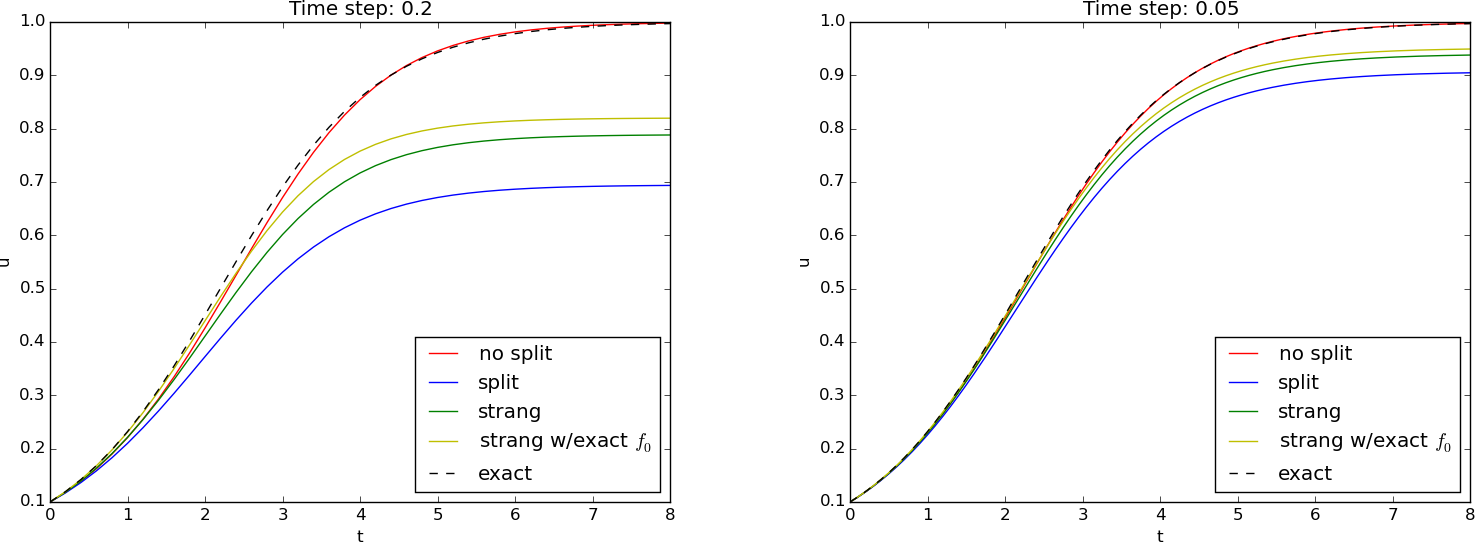
5.33 Reaction-diffusion equation
Consider a diffusion equation coupled to chemical reactions modeled by a nonlinear term \(f(u)\): \[ \frac{\partial u}{\partial t} = \dfc\nabla^2u + f(u)\tp \] This is a physical process composed of two individual processes: \(u\) is the concentration of a substance that is locally generated by a chemical reaction \(f(u)\), while \(u\) is spreading in space because of diffusion. There are obviously two time scales: one for the chemical reaction and one for diffusion. Typically, fast chemical reactions require much finer time stepping than slower diffusion processes. It could therefore be advantageous to split the two physical effects in separate models and use different numerical methods for the two.
A natural spitting in the present case is
\[ \frac{\partial u^{\stepzero}}{\partial t} = \dfc\nabla^2 u^{\stepzero}, \] \[ \frac{\partial u^{\stepone}}{\partial t} = f(u^{\stepone})\tp \tag{5.40}\] Looking at these familiar problems, we may apply a \(\theta\) rule (implicit) scheme for (5.40) over one time step and avoid dealing with nonlinearities by applying an explicit scheme for (5.40) over the same time step.
Suppose we have some solution \(u\) at time level \(t_n\). For flexibility, we define a \(\theta\) method for the diffusion part (5.40) by \[ [D_t u^\stepzero = \dfc (D_xD_x u^\stepzero + D_y D_y u^\stepzero)]^{n+\theta}\tp \] We use \(u^{n}\) as initial condition for \(u^\stepzero\).
The reaction part, which is defined at each mesh point (without coupling values in different mesh points), can employ any scheme for an ODE. Here we use an Adams-Bashforth method of order 2. Recall that the overall accuracy of the splitting method is maximum \(\Oof{\Delta t^2}\) for Strange splitting, otherwise it is just \(\Oof{\Delta t}\). Higher-order methods for ODEs will therefore be a waste of work. The 2nd-order Adams-Bashforth method reads \[ u^{\stepone,n+1}_{i,j} = u^{\stepone,n}_{i,j} + \half\Delta t\left( 3f(u^{\stepone, n}_{i,j}, t_n) - f(u^{\stepone, n-1}_{i,j}, t_{n-1}) \right) \tp \] We can use a Forward Euler step to start the method, i.e, compute \(u^{\stepone,1}_{i,j}\).
The algorithm goes like this:
- Solve the diffusion problem for one time step as usual.
- Solve the reaction ODEs at each mesh point in \([t_n,t_n+\Delta t]\), using the diffusion solution in 1. as initial condition. The solution of the ODEs constitutes the solution of the original problem at the end of each time step.
We may use a much smaller time step when solving the reaction part, adapted to the dynamics of the problem \(u'=f(u)\). This gives great flexibility in splitting methods.
5.34 Example: Reaction-Diffusion with linear reaction term
The methods above may be explored in detail through a specific computational example in which we compute the convergence rates associated with four different solution approaches for the reaction-diffusion equation with a linear reaction term, i.e. \(f(u)=-bu\). The methods comprise solving without splitting (just straight Forward Euler), ordinary splitting, first order Strange splitting, and second order Strange splitting. In all four methods, a standard centered difference approximation is used for the spatial second derivative. The methods share the error model \(E = C h^r\), while differing in the step \(h\) (being either \(\Delta x^2\) or \(\Delta x\)) and the convergence rate \(r\) (being either 1 or 2).
All code commented below is found in the file split_diffu_react.py.
The code in this section has been refactored into testable source files. See src/nonlin/split_diffu_react.py for the complete implementation, which is exercised by the test suite. The code shown below is adapted from that source to match the original presentation style.
When executed, a function convergence_rates is called, from which all convergence rate computations are handled:
def convergence_rates(scheme="diffusion"):
    """Computes empirical conv. rates for the different
    splitting schemes"""

    F = 0.5
    T = 1.2
    a = 3.5
    b = 1
    L = 1.5
    k = np.pi / L

    def exact(x, t):
        """exact sol. to: du/dt = a*d^2u/dx^2 - b*u"""
        return np.exp(-(a * k**2 + b) * t) * np.sin(k * x)

    def f(u, t):
        return -b * u

    def I(x):
        return exact(x, 0)

    global error  # error computed in the user action function
    error = 0

    def action(u, x, t, n):
        global error
        if n == 1:  # New simulation, - reset error
            error = 0
        else:
            error = max(error, np.abs(u - exact(x, t[n])).max())

    E = []
    h = []
    Nx_values = [10, 20, 40, 80, 160]
    for Nx in Nx_values:
        dx = L / Nx
        dt = F / a * dx**2
        Nt = int(round(T / float(dt)))
        t = np.linspace(0, Nt * dt, Nt + 1)  # Mesh points, global time

        if scheme == "diffusion":
            print("Running FE on whole eqn...")
            diffusion_FE(I, a, f, L, dt, F, t, T, step_no=0, user_action=action)
        elif scheme == "ordinary_splitting":
            print("Running ordinary splitting...")
            ordinary_splitting(
                I=I,
                a=a,
                b=b,
                f=f,
                L=L,
                dt=dt,
                dt_Rfactor=1,
                F=F,
                t=t,
                T=T,
                user_action=action,
            )
        elif scheme == "Strange_splitting_1stOrder":
            print("Running Strange splitting with 1st order schemes...")
            Strange_splitting_1stOrder(
                I=I,
                a=a,
                b=b,
                f=f,
                L=L,
                dt=dt,
                dt_Rfactor=1,
                F=F,
                t=t,
                T=T,
                user_action=action,
            )
        elif scheme == "Strange_splitting_2andOrder":
            print("Running Strange splitting with 2nd order schemes...")
            Strange_splitting_2andOrder(
                I=I,
                a=a,
                b=b,
                f=f,
                L=L,
                dt=dt,
                dt_Rfactor=1,
                F=F,
                t=t,
                T=T,
                user_action=action,
            )
        else:
            print("Unknown scheme requested!")
            sys.exit(0)

        h.append(dt)
        E.append(error)

    print("E:", E)
    print("h:", h)

    r = [
        np.log(E[i] / E[i - 1]) / np.log(h[i] / h[i - 1])
        for i in range(1, len(Nx_values))
    ]
    print("Computed rates:", r)


if __name__ == "__main__":
    schemes = [
        "diffusion",
        "ordinary_splitting",
        "Strange_splitting_1stOrder",
        "Strange_splitting_2andOrder",
    ]

    for scheme in schemes:
        convergence_rates(scheme=scheme)
Now, with respect to the error (\(E = C h^r\)), the Forward Euler scheme, the ordinary splitting scheme and first order Strange splitting scheme are all first order (\(r = 1\)), with a step \(h = \Delta x^2 =
K^{-1}\Delta t\), where \(K\) is some constant. This implies that the ratio \(\frac{\Delta t}{\Delta x^2}\) must be held constant during convergence rate calculations. Furthermore, the Fourier number \(F =
\frac{\alpha \Delta t}{\Delta x^2}\) is upwards limited to \(F = 0.5\), being the stability limit with explicit schemes. Thus, in these cases, we use the fixed value of \(F\) and a given (but changing) spatial resolution \(\Delta x\) to compute the corresponding value of \(\Delta t\) according to the expression for \(F\). This assures that \(\frac{\Delta
t}{\Delta x^2}\) is kept constant. The loop in convergence_rates runs over a chosen set of grid points (Nx_values) which gives a doubling of spatial resolution with each iteration (\(\Delta x\) is halved).
For the second order Strange splitting scheme, we have \(r = 2\) and a step \(h = \Delta x = K^{-1}\Delta t\), where \(K\) again is some constant. In this case, it is thus the ratio \(\frac{\Delta t}{\Delta x}\) that must be held constant during the convergence rate calculations. From the expression for \(F\), it is clear then that \(F\) must change with each halving of \(\Delta x\). In fact, if \(F\) is doubled each time \(\Delta x\) is halved, the ratio \(\frac{\Delta t}{\Delta x}\) will be constant (this follows, e.g., from the expression for \(F\)). This is utilized in our code.
A solver diffusion_theta is used in each of the four solution approaches:
def diffusion_theta(
    I, a, f, L, dt, F, t, T, step_no, theta=0.5, u_L=0, u_R=0, user_action=None
):
    """
    Full solver for the model problem using the theta-rule
    difference approximation in time (no restriction on F,
    i.e., the time step when theta >= 0.5).
    Vectorized implementation and sparse (tridiagonal)
    coefficient matrix.
    """

    Nt = int(round(T / float(dt)))
    dx = np.sqrt(a * dt / F)
    Nx = int(round(L / dx))
    x = np.linspace(0, L, Nx + 1)  # Mesh points in space
    dx = x[1] - x[0]
    dt = t[1] - t[0]

    u = np.zeros(Nx + 1)  # solution array at t[n+1]
    u_1 = np.zeros(Nx + 1)  # solution at t[n]

    diagonal = np.zeros(Nx + 1)
    lower = np.zeros(Nx)
    upper = np.zeros(Nx)
    b = np.zeros(Nx + 1)

    Fl = F * theta
    Fr = F * (1 - theta)
    diagonal[:] = 1 + 2 * Fl
    lower[:] = -Fl  # 1
    upper[:] = -Fl  # 1
    diagonal[0] = 1
    upper[0] = 0
    diagonal[Nx] = 1
    lower[-1] = 0

    diags = [0, -1, 1]
    A = scipy.sparse.diags(
        diagonals=[diagonal, lower, upper],
        offsets=[0, -1, 1],
        shape=(Nx + 1, Nx + 1),
        format="csr",
    )

    if f is None or f == 0:
        f = lambda x, t: np.zeros(x.size) if isinstance(x, np.ndarray) else 0

    if isinstance(I, np.ndarray):  # I is an array
        u_1 = np.copy(I)
    else:  # I is a function
        for i in range(0, Nx + 1):
            u_1[i] = I(x[i])

    if user_action is not None:
        user_action(u_1, x, t, step_no + 0)

    for n in range(0, Nt):
        b[1:-1] = (
            u_1[1:-1]
            + Fr * (u_1[:-2] - 2 * u_1[1:-1] + u_1[2:])
            + dt * theta * f(u_1[1:-1], t[step_no + n + 1])
            + dt * (1 - theta) * f(u_1[1:-1], t[step_no + n])
        )
        b[0] = u_L
        b[-1] = u_R  # boundary conditions
        u[:] = scipy.sparse.linalg.spsolve(A, b)

        if user_action is not None:
            user_action(u, x, t, step_no + (n + 1))

        u_1, u = u, u_1

    return u_1
For the no splitting approach with Forward Euler in time, this solver handles both the diffusion and the reaction term. When splitting, diffusion_theta takes care of the diffusion term only, while the reaction term is handled either by a Forward Euler scheme in reaction_FE, or by a second order Adams-Bashforth scheme from Odespy. The reaction_FE function covers one complete time step dt during ordinary splitting, while Strange splitting (both first and second order) applies it with dt/2 twice during each time step dt. Since the reaction term typically represents a much faster process than the diffusion term, a further refinement of the time step is made possible in reaction_FE. It was implemented as
def reaction_FE(I, f, L, Nx, dt, dt_Rfactor, t, step_no, user_action=None):
    """Reaction solver, Forward Euler method.
    Note that t covers the whole global time interval.
    dt is the step of the diffustion part, i.e. there
    is a local time interval [0, dt] the reaction_FE
    deals with each time it is called. step_no keeps
    track of the (global) time step number (required
    for lookup in t).
    """


    u = np.copy(I)
    dt_local = dt / float(dt_Rfactor)
    Nt_local = int(round(dt / float(dt_local)))
    x = np.linspace(0, L, Nx + 1)

    for n in range(Nt_local):
        time = t[step_no] + n * dt_local
        u[1:Nx] = u[1:Nx] + dt_local * f(u[1:Nx], time)


    return u
With the ordinary splitting approach, each time step dt is covered twice. First computing the impact of the reaction term, then the contribution from the diffusion term:
def ordinary_splitting(I, a, b, f, L, dt, dt_Rfactor, F, t, T, user_action=None):
    """1st order scheme, i.e. Forward Euler is enough for both
    the diffusion and the reaction part. The time step dt is
    given for the diffusion step, while the time step for the
    reaction part is found as dt/dt_Rfactor, where dt_Rfactor >= 1.
    """
    Nt = int(round(T / float(dt)))
    dx = np.sqrt(a * dt / F)
    Nx = int(round(L / dx))
    x = np.linspace(0, L, Nx + 1)  # Mesh points in space
    u = np.zeros(Nx + 1)

    for i in range(0, Nx + 1):
        u[i] = I(x[i])

    for n in range(0, Nt):

        u_s = diffusion_FE(
            I=u, a=a, f=0, L=L, dt=dt, F=F, t=t, T=dt, step_no=n, user_action=None
        )
        u = reaction_FE(
            I=u_s,
            f=f,
            L=L,
            Nx=Nx,
            dt=dt,
            dt_Rfactor=dt_Rfactor,
            t=t,
            step_no=n,
            user_action=None,
        )

        if user_action is not None:
            user_action(u, x, t, n + 1)
For the two Strange splitting approaches, each time step dt is handled by first computing the reaction step for (the first) dt/2, followed by a diffusion step dt, before the reaction step is treated once again for (the remaining) dt/2. Since first order Strange splitting is no better than first order accurate, both the reaction and diffusion steps are computed explicitly. The solver was implemented as
def Strange_splitting_1stOrder(I, a, b, f, L, dt, dt_Rfactor, F, t, T, user_action=None):
    """Strange splitting while still using FE for the diffusion
    step and for the reaction step. Gives 1st order scheme.
    Introduce an extra time mesh t2 for the diffusion part,
    since it steps dt/2.
    """
    Nt = int(round(T / float(dt)))
    t2 = np.linspace(0, Nt * dt, (Nt + 1) + Nt)  # Mesh points in diff
    dx = np.sqrt(a * dt / F)
    Nx = int(round(L / dx))
    x = np.linspace(0, L, Nx + 1)
    u = np.zeros(Nx + 1)

    for i in range(0, Nx + 1):
        u[i] = I(x[i])

    for n in range(0, Nt):
        u_s = diffusion_FE(
            I=u,
            a=a,
            f=0,
            L=L,
            dt=dt / 2.0,
            F=F / 2.0,
            t=t2,
            T=dt / 2.0,
            step_no=2 * n,
            user_action=None,
        )

        u_sss = reaction_FE(
            I=u_s,
            f=f,
            L=L,
            Nx=Nx,
            dt=dt,
            dt_Rfactor=dt_Rfactor,
            t=t,
            step_no=n,
            user_action=None,
        )

        u = diffusion_FE(
            I=u_sss,
            a=a,
            f=0,
            L=L,
            dt=dt / 2.0,
            F=F / 2.0,
            t=t2,
            T=dt / 2.0,
            step_no=2 * n + 1,
            user_action=None,
        )

        if user_action is not None:
            user_action(u, x, t, n + 1)
The second order version of the Strange splitting approach utilizes a second order Adams-Bashforth solver for the reaction part and a Crank-Nicolson scheme for the diffusion part. The solver has the same structure as the one for first order Strange splitting and was implemented as
def Strange_splitting_2andOrder(I, a, b, f, L, dt, dt_Rfactor, F, t, T, user_action=None):
    """Strange splitting using Crank-Nicolson for the diffusion
    step (theta-rule) and Adams-Bashforth 2 for the reaction step.
    Gives 2nd order scheme. Introduce an extra time mesh t2 for
    the diffusion part, since it steps dt/2.
    """
    import odespy

    Nt = int(round(T / float(dt)))
    t2 = np.linspace(0, Nt * dt, (Nt + 1) + Nt)  # Mesh points in diff
    dx = np.sqrt(a * dt / F)
    Nx = int(round(L / dx))
    x = np.linspace(0, L, Nx + 1)
    u = np.zeros(Nx + 1)

    for i in range(0, Nx + 1):
        u[i] = I(x[i])

    reaction_solver = odespy.AdamsBashforth2(f)

    for n in range(0, Nt):
        u_s = diffusion_theta(
            I=u,
            a=a,
            f=0,
            L=L,
            dt=dt / 2.0,
            F=F / 2.0,
            t=t2,
            T=dt / 2.0,
            step_no=2 * n,
            theta=0.5,
            u_L=0,
            u_R=0,
            user_action=None,
        )


        reaction_solver.set_initial_condition(u_s)
        t_points = np.linspace(0, dt, dt_Rfactor + 1)
        u_AB2, t_ = reaction_solver.solve(t_points)  # t_ not needed
        u_sss = u_AB2[-1, :]  # pick sol at last point in time


        u = diffusion_theta(
            I=u_sss,
            a=a,
            f=0,
            L=L,
            dt=dt / 2.0,
            F=F / 2.0,
            t=t2,
            T=dt / 2.0,
            step_no=2 * n + 1,
            theta=0.5,
            u_L=0,
            u_R=0,
            user_action=None,
        )


        if user_action is not None:
            user_action(u, x, t, n + 1)
When executing split_diffu_react.py, we find that the estimated convergence rates are as expected. The second order Strange splitting gives the least error (about \(4e^{-5}\)) and has second order convergence (\(r = 2\)), while the remaining three approaches have first order convergence (\(r = 1\)).
5.35 Analysis of the splitting method
Let us address a linear PDE problem for which we can develop analytical solutions of the discrete equations, with and without splitting, and discuss these. Choosing \(f(u)=-\beta u\) for a constant \(\beta\) gives a linear problem. We use the Forward Euler method for both the PDE and ODE problems.
We seek a 1D Fourier wave component solution of the problem, assuming homogeneous Dirichlet conditions at \(x=0\) and \(x=L\): \[ u = e^{-\dfc k^2 t - \beta t}\sin kx,\quad k = \frac{\pi}{L}\tp \] This component fits the 1D PDE problem (\(f=0\)). On complex form we can write \[ u = e^{-\dfc k^2 t - \beta t + ikx}, \] where \(i=\sqrt{-1}\) and the imaginary part is taken as the physical solution.
We refer to Section 3.15 and to the book (Langtangen 2016) for a discussion of exact numerical solutions to diffusion and decay problems, respectively. The key idea is to search for solutions \(A^ne^{ikx}\) and determine \(A\). For the diffusion problem solved by a Forward Euler method one has \[ A = 1 - 4F\sin^p, \] where \(F=\dfc\Delta t/\Delta x^2\) is the mesh Fourier number and \(p=k\Delta x/2\) is a dimensionless number reflecting the spatial resolution (number of points per wave length in space). For the decay problem \(u'=-\beta u\), we have \(A=1 - q\), where \(q\) is a dimensionless parameter for the resolution in the decay problem: \(q = \beta\Delta t\).
The original model problem can also be discretized by a Forward Euler scheme, \[ [D^+_t u = \dfc D_xD_x u - \beta u]^n_i\tp \] Assuming \(A^ne^{ikx}\) we find that \[ u^n_i = (1 - 4F\sin^p -q)^n\sin kx\tp \] We are particularly interested in what happens at one time step. That is, \[ u^{n}_{i} = (1-4F\sin^2 p)u^{n-1}_i\tp \] In the two stage algorithm, we first compute the diffusion step \[ u^{\stepzero,n+1}_i = (1 - 4F\sin^2 p)u^{n-1}_i\tp \] Then we use this as input to the decay algorithm and arrive at \[ u^{\stepone,n+1} = (1-q)u^{\stepzero,n+1} = (1-q)(1-4F\sin^2 p) u^{n-1}_i\tp \] The splitting approximation over one step is therefore \[ E = 1 - 4F\sin^p -q - (1-q)(1-4F\sin^2 p) = -q(2 - F\sin^2 p))\tp \]
5.36 Problem: Determine if equations are nonlinear or not
Classify each term in the following equations as linear or nonlinear. Assume that \(u\), \(\uu\), and \(p\) are unknown functions and that all other symbols are known quantities.
- \(mu^{\prime\prime} + \beta |u^{\prime}|u^{\prime} + cu = F(t)\)
- \(u_t = \dfc u_{xx}\)
- \(u_{tt} = c^2\nabla^2 u\)
- \(u_t = \nabla\cdot(\dfc(u)\nabla u) + f(x,y)\)
- \(u_t + f(u)_x = 0\)
- \(\uu_t + \uu\cdot\nabla \uu = -\nabla p + r\nabla^2\uu\), \(\nabla\cdot\uu = 0\) (\(\uu\) is a vector field)
- \(u^{\prime} = f(u,t)\)
- \(\nabla^2 u = \lambda e^u\)
- \(mu^{\prime\prime}\) is linear; \(\beta |u^{\prime}|u^{\prime}\) is nonlinear; \(cu\) is linear; \(F(t)\) does not contain the unknown \(u\) and is hence constant in \(u\), so the term is linear.
- \(u_t\) is linear; \(\dfc u_{xx}\) is linear.
- \(u_{tt}\) is linear; \(c^2\nabla^2 u\) is linear.
- \(u_t\) is linear; \(\nabla\cdot(\dfc(u)\nabla u)\) is nonlinear; \(f(x,y)\) is constant in \(u\) and hence linear.
- \(u_t\) is linear; \(f(u)_x\) is nonlinear if \(f\) is nonlinear in \(u\).
- \(\uu_t\) is linear; \(\uu\cdot\nabla \uu\) is nonlinear; \(-\nabla p\) is linear (in \(p\)); \(r\nabla^2\uu\) is linear; \(\nabla\cdot\uu\) is linear.
- \(u^{\prime}\) is linear; \(f(u,t)\) is nonlinear if \(f\) is nonlinear in \(u\).
- \(\nabla^2 u\) is linear; \(\lambda e^u\) is nonlinear.
5.37 Exercise: Derive a relaxation formula
Derive (5.9) in Section Section 5.9.
5.38 Problem: Derive and investigate a generalized logistic model
The logistic model for population growth is derived by assuming a nonlinear growth rate, \[ u^{\prime} = a(u)u,\quad u(0)=I, \tag{5.41}\] and the logistic model arises from the simplest possible choice of \(a(u)\): \(r(u)=\varrho(1 - u/M)\), where \(M\) is the maximum value of \(u\) that the environment can sustain, and \(\varrho\) is the growth under unlimited access to resources (as in the beginning when \(u\) is small). The idea is that \(a(u)\sim\varrho\) when \(u\) is small and that \(a(t)\rightarrow 0\) as \(u\rightarrow M\).
An \(a(u)\) that generalizes the linear choice is the polynomial form \[ a(u) = \varrho(1-u/M)^p, \tag{5.42}\] where \(p>0\) is some real number.
a)
Formulate a Forward Euler, Backward Euler, and a Crank-Nicolson scheme for (5.41).
\([a(u)u]^{n+1/2}\approx a(u^n)u^{n+1}\).
The Forward Euler scheme reads \[ [D^+_t u = a(u)u]^n, \] or written out, \[ \frac{u^{n+1}-u^n}{\Delta t} = a(u^n)u^n\tp \] The scheme is linear in the unknown \(u^{n+1}\): \[ u^{n+1} = u^n + {\Delta t}a(u^n)u^n\tp \] The Backward Euler scheme, \[ [D^-_t u = a(u)u]^n, \] becomes \[ \frac{u^{n}-u^{n-1}}{\Delta t} = a(u^n)u^n, \] which is a nonlinear equation in the unknown \(u\), here expressed as \(u^{n+1}\): \[ u^{n+1} - \Delta t a(u^{n+1})u^{n+1} = u^n\tp \] The standard Crank-Nicolson scheme, \[ D_t u = \overline{a(u)u}^t]^{n+\half}, \] takes the form \[ \frac{u^{n+1}-u^n}{\Delta t} = \half a(u^n)u^n + \half a(u^{n+1})u^{n+1}\tp \] This is a nonlinear equation in the unknown \(u^{n+1}\), \[ u^{n+1} - \half {\Delta t} a(u^{n+1})u^{n+1} = u^n + \half {\Delta t} a(u^n)u^n\tp \] However, with the suggested geometric mean, the \(a(u)u\) term is linearized: \[ \frac{u^{n+1}-u^n}{\Delta t} = a(u^n)u^{n+1}, \] leading to a linear equation in \(u^{n+1}\): \[ (1 - \Delta t a(u^n))u^{n+1} = u^n\tp \]
b)
Formulate Picard and Newton iteration for the Backward Euler scheme in a).
A Picard iteration for \[ u^{n+1} - \Delta t a(u^{n+1})u^{n+1} = u^n\tp \] applies old values in for \(u^{n+1}\) in \(a(u^{n+1})\). If \(u^-\) is the most recently computed approximation to \(u^{n+1}\), we can write the Picard linearization as \[ (1 - \Delta t a(u^-))u^{n+1} = u^n\tp \] Alternatively, with an iteration index \(k\), \[ (1 - \Delta t a(u^{n+1,k}))u^{n+1,k+1} = u^n\tp \] Newton’s method starts with identifying the nonlinear equation as \(F(u)=0\), and here \[ F(u) = u - \Delta t a(u)u - u^n\tp \] The Jacobian is \[ J(u) = \frac{F(u)}{du} = 1 - \Delta t(a'(u)u + a(u))\tp \] The key equation in Newton’s method is then \[ J(u^-)\delta u = - F(u^-),\quad u\leftarrow u - \delta u\tp \]
c)
Implement the numerical solution methods from a) and b). Use logistic.py to compare the case \(p=1\) and the choice (5.42).
We specialize the code for \(a(u)\) to (5.42) since the code was developed from logistic.py. It is convenient to work with a dimensionless form of the problem. Choosing a time scale \(t_c = 1\varrho\) and a scale for \(u\), \(u_c=M\), leads to \[
u^{\prime} = \varrho (1-u)^p u,\quad u(0)=\alpha,
\] where \(\alpha\) is a dimensionless number \[
\alpha = \frac{I}{M}\tp
\] The three schemes can be implemented as follows.
import numpy as np


def FE_logistic(p, u0, dt, Nt):
    u = np.zeros(Nt + 1)
    u[0] = u0
    for n in range(Nt):
        u[n + 1] = u[n] + dt * (1 - u[n]) ** p * u[n]
    return u


def BE_logistic(p, u0, dt, Nt, choice="Picard", eps_r=1e-3, omega=1, max_iter=1000):
    if choice == "Picard1":
        choice = "Picard"
        max_iter = 1

    u = np.zeros(Nt + 1)
    iterations = []
    u[0] = u0
    for n in range(1, Nt + 1):
        c = -u[n - 1]
        if choice == "Picard":

            def F(u):
                return -dt * (1 - u) ** p * u + u + c

            u_ = u[n - 1]
            k = 0
            while abs(F(u_)) > eps_r and k < max_iter:
                u_ = omega * (-c / (1 - dt * (1 - u_) ** p)) + (1 - omega) * u_
                k += 1
            u[n] = u_
            iterations.append(k)

        elif choice == "Newton":

            def F(u):
                return -dt * (1 - u) ** p * u + u + c

            def dF(u):
                return dt * p * (1 - u) ** (p - 1) * u - dt * (1 - u) ** p + 1

            u_ = u[n - 1]
            k = 0
            while abs(F(u_)) > eps_r and k < max_iter:
                u_ = u_ - F(u_) / dF(u_)
                k += 1
            u[n] = u_
            iterations.append(k)
    return u, iterations


def CN_logistic(p, u0, dt, Nt):
    u = np.zeros(Nt + 1)
    u[0] = u0
    for n in range(0, Nt):
        u[n + 1] = u[n] / (1 - dt * (1 - u[n]) ** p)
    return u
A first verification is to choose \(p=1\) and compare the results with those from logistic.py. The number of iterations and the final numerical answers should be identical.
d)
Implement unit tests that check the asymptotic limit of the solutions: \(u\rightarrow M\) as \(t\rightarrow\infty\).
(increases substantially with \(p\)) and what the appropriate tolerance is for testing the asymptotic limit.
The test function may look like
def test_asymptotic_value():
    T = 100
    dt = 0.1
    Nt = int(round(T / float(dt)))
    u0 = 0.1
    p = 1.8

    u_CN = CN_logistic(p, u0, dt, Nt)
    u_BE_Picard, iter_Picard = BE_logistic(
        p, u0, dt, Nt, choice="Picard", eps_r=1e-5, omega=1, max_iter=1000
    )
    u_BE_Newton, iter_Newton = BE_logistic(
        p, u0, dt, Nt, choice="Newton", eps_r=1e-5, omega=1, max_iter=1000
    )
    u_FE = FE_logistic(p, u0, dt, Nt)

    for arr in u_CN, u_BE_Picard, u_BE_Newton, u_FE:
        expected = 1
        computed = arr[-1]
        tol = 0.01
        msg = f"expected={expected}, computed={computed}"
        print(msg)
        assert abs(expected - computed) < tol
It is important with a sufficiently small eps_r tolerance for the asymptotic value to be accurate (using eps_r=1E-3 leads to a value 0.92 at \(t=T\) instead of 0.994 when eps_r=1E-5).
e)
Perform experiments with Newton and Picard iteration for the model (5.42). See how sensitive the number of iterations is to \(\Delta t\) and \(p\).
Appropriate code is
import matplotlib.pyplot as plt


def demo():
    T = 12
    p = 1.2
    try:
        dt = float(sys.argv[1])
        eps_r = float(sys.argv[2])
        omega = float(sys.argv[3])
    except:
        dt = 0.8
        eps_r = 1e-3
        omega = 1
    N = int(round(T / float(dt)))

    u_FE = FE_logistic(p, 0.1, dt, N)
    u_BE31, iter_BE31 = BE_logistic(p, 0.1, dt, N, "Picard1", eps_r, omega)
    u_BE3, iter_BE3 = BE_logistic(p, 0.1, dt, N, "Picard", eps_r, omega)
    u_BE4, iter_BE4 = BE_logistic(p, 0.1, dt, N, "Newton", eps_r, omega)
    u_CN = CN_logistic(p, 0.1, dt, N)

    print(f"Picard mean no of iterations (dt={dt:g}):", int(round(np.mean(iter_BE3))))
    print(f"Newton mean no of iterations (dt={dt:g}):", int(round(np.mean(iter_BE4))))

    t = np.linspace(0, dt * N, N + 1)
    plt.figure()
    plt.plot(t, u_FE, label="FE")
    plt.plot(t, u_BE3, label="BE Picard")
    plt.plot(t, u_BE31, label="BE Picard1")
    plt.plot(t, u_BE4, label="BE Newton")
    plt.plot(t, u_CN, label="CN gm")
    plt.legend(loc="lower right")
    plt.title(f"dt={dt:g}, eps={eps_r:.0E}")
    plt.xlabel("t")
    plt.ylabel("u")
    filestem = "logistic_N%d_eps%03d" % (N, np.log10(eps_r))
    plt.savefig(filestem + "_u.png")
    plt.savefig(filestem + "_u.pdf")

    plt.figure()
    plt.plot(range(1, len(iter_BE3) + 1), iter_BE3, "r-o", label="Picard")
    plt.plot(range(1, len(iter_BE4) + 1), iter_BE4, "b-o", label="Newton")
    plt.legend()
    plt.title(f"dt={dt:g}, eps={eps_r:.0E}")
    plt.axis([1, N + 1, 0, max(iter_BE3 + iter_BE4) + 1])
    plt.xlabel("Time level")
    plt.ylabel("No of iterations")
    plt.savefig(filestem + "_iter.png")
    plt.savefig(filestem + "_iter.pdf")
5.39 Problem: Experience the behavior of Newton’s method
The program Newton_demo.py illustrates graphically each step in Newton’s method and is run like
Terminal> python Newton_demo.py f dfdx x0 xmin xmaxUse this program to investigate potential problems with Newton’s method when solving \(e^{-0.5x^2}\cos (\pi x)=0\). Try a starting point \(x_0=0.8\) and \(x_0=0.85\) and watch the different behavior. Just run
Terminal>  python Newton_demo.py '0.2 + exp(-0.5*x**2)*cos(pi*x)' \
           '-x*exp(-x**2)*cos(pi*x) - pi*exp(-x**2)*sin(pi*x)' \
           0.85 -3 3
and repeat with 0.85 replaced by 0.8.
5.40 Exercise: Compute the Jacobian of a \(2\times 2\) system
Write up the system (5.13)-(5.14) in the form \(F(u)=0\), \(F=(F_0,F_1)\), \(u=(u_0,u_1)\), and compute the Jacobian \(J_{i,j}=\partial F_i/\partial u_j\).
5.41 Problem: Solve nonlinear equations arising from a vibration ODE
Consider a nonlinear vibration problem \[ mu^{\prime\prime} + bu^{\prime}|u^{\prime}| + s(u) = F(t), \] where \(m>0\) is a constant, \(b\geq 0\) is a constant, \(s(u)\) a possibly nonlinear function of \(u\), and \(F(t)\) is a prescribed function. Such models arise from Newton’s second law of motion in mechanical vibration problems where \(s(u)\) is a spring or restoring force, \(mu^{\prime\prime}\) is mass times acceleration, and \(bu^{\prime}|u^{\prime}|\) models water or air drag.
a)
Rewrite the equation for \(u\) as a system of two first-order ODEs, and discretize this system by a Crank-Nicolson (centered difference) method. With \(v=u^\prime\), we get a nonlinear term \(v^{n+\frac{1}{2}}|v^{n+\frac{1}{2}}|\). Use a geometric average for \(v^{n+\frac{1}{2}}\).
b)
Formulate a Picard iteration method to solve the system of nonlinear algebraic equations.
c)
Explain how to apply Newton’s method to solve the nonlinear equations at each time level. Derive expressions for the Jacobian and the right-hand side in each Newton iteration.
5.42 Exercise: Find the truncation error of arithmetic mean of products
In Section Section 5.21 we introduce alternative arithmetic means of a product. Say the product is \(P(t)Q(t)\) evaluated at \(t=t_{n+\frac{1}{2}}\). The exact value is \[ [PQ]^{n+\frac{1}{2}} = P^{n+\frac{1}{2}}Q^{n+\frac{1}{2}} \] There are two obvious candidates for evaluating \([PQ]^{n+\frac{1}{2}}\) as a mean of values of \(P\) and \(Q\) at \(t_n\) and \(t_{n+1}\). Either we can take the arithmetic mean of each factor \(P\) and \(Q\), \[ [PQ]^{n+\frac{1}{2}} \approx \frac{1}{2}(P^n + P^{n+1})\frac{1}{2}(Q^n + Q^{n+1}), \tag{5.43}\] or we can take the arithmetic mean of the product \(PQ\): \[ [PQ]^{n+\frac{1}{2}} \approx \frac{1}{2}(P^nQ^n + P^{n+1}Q^{n+1})\tp \tag{5.44}\]
The arithmetic average of \(P(t_{n+\frac{1}{2}})\) is \(\Oof{\Delta t^2}\): \[ P(t_{n+\frac{1}{2}}) = \frac{1}{2}(P^n + P^{n+1}) +\Oof{\Delta t^2}\tp \] A fundamental question is whether (5.43) and (5.44) have different orders of accuracy in \(\Delta t = t_{n+1}-t_n\). To investigate this question, expand quantities at \(t_{n+1}\) and \(t_n\) in Taylor series around \(t_{n+\frac{1}{2}}\), and subtract the true value \([PQ]^{n+\frac{1}{2}}\) from the approximations (5.43) and (5.44) to see what the order of the error terms are.
sympy for carrying out the tedious calculations.
A general Taylor series expansion of \(P(t+\frac{1}{2}\Delta t)\) around \(t\) involving just a general function \(P(t)\) can be created as follows:
>>> from sympy import *
>>> t, dt = symbols('t dt')
>>> P = symbols('P', cls=Function)
>>> P(t).series(t, 0, 4)
P(0) + t*Subs(Derivative(P(_x), _x), (_x,), (0,)) +
t**2*Subs(Derivative(P(_x), _x, _x), (_x,), (0,))/2 +
t**3*Subs(Derivative(P(_x), _x, _x, _x), (_x,), (0,))/6 + O(t**4)
>>> P_p = P(t).series(t, 0, 4).subs(t, dt/2)
>>> P_p
P(0) + dt*Subs(Derivative(P(_x), _x), (_x,), (0,))/2 +
dt**2*Subs(Derivative(P(_x), _x, _x), (_x,), (0,))/8 +
dt**3*Subs(Derivative(P(_x), _x, _x, _x), (_x,), (0,))/48 + O(dt**4)
The error of the arithmetic mean, \(\frac{1}{2}(P(-\frac{1}{2}\Delta t) + P(-\frac{1}{2}\Delta t))\) for \(t=0\) is then
>>> P_m = P(t).series(t, 0, 4).subs(t, -dt/2)
>>> mean = Rational(1,2)*(P_m + P_p)
>>> error = simplify(expand(mean) - P(0))
>>> error
dt**2*Subs(Derivative(P(_x), _x, _x), (_x,), (0,))/8 + O(dt**4)
Use these examples to investigate the error of (5.43) and (5.44) for \(n=0\). (Choosing \(n=0\) is necessary for not making the expressions too complicated for sympy, but there is of course no lack of generality by using \(n=0\) rather than an arbitrary \(n\) - the main point is the product and addition of Taylor series.)
5.43 Problem: Newton’s method for linear problems
Suppose we have a linear system \(F(u) = Au- b=0\). Apply Newton’s method to this system, and show that the method converges in one iteration.
5.44 Problem: Discretize a 1D problem with a nonlinear coefficient
We consider the problem \[ ((1 + u^2)u^{\prime})^{\prime} = 1,\quad x\in (0,1),\quad u(0)=u(1)=0\tp \tag{5.45}\]
Discretize (5.45) by a centered finite difference method on a uniform mesh.
5.45 Problem: Linearize a 1D problem with a nonlinear coefficient
We have a two-point boundary value problem \[ ((1 + u^2)u^{\prime})^{\prime} = 1,\quad x\in (0,1),\quad u(0)=u(1)=0\tp \tag{5.46}\]
a)
Construct a Picard iteration method for (5.46) without discretizing in space.
b)
Apply Newton’s method to (5.46) without discretizing in space.
c)
Discretize (5.46) by a centered finite difference scheme. Construct a Picard method for the resulting system of nonlinear algebraic equations.
d)
Discretize (5.46) by a centered finite difference scheme. Define the system of nonlinear algebraic equations, calculate the Jacobian, and set up Newton’s method for solving the system.
5.46 Problem: Finite differences for the 1D Bratu problem
5.47 Good: http://faculty.oxy.edu/ron/research/bratu/bratu.pdf
5.48 It has a collocation method too
We address the so-called Bratu problem \[ u^{\prime\prime} + \lambda e^u=0,\quad x\in (0,1),\quad u(0)=u(1)=0, \tag{5.47}\] where \(\lambda\) is a given parameter and \(u\) is a function of \(x\). This is a widely used model problem for studying numerical methods for nonlinear differential equations. The problem (5.47) has an exact solution \[ u_{\text{e}}(x) = -2\ln\left(\frac{\cosh((x-\half)\theta/2)}{\cosh(\theta/4)}\right), \] where \(\theta\) solves \[ \theta = \sqrt{2\lambda}\cosh(\theta/4)\tp \] There are two solutions of (5.47) for \(0<\lambda <\lambda_c\) and no solution for \(\lambda >\lambda_c\). For \(\lambda = \lambda_c\) there is one unique solution. The critical value \(\lambda_c\) solves \[ 1 = \sqrt{2\lambda_c}\frac{1}{4}\sinh(\theta(\lambda_c)/4)\tp \] A numerical value is \(\lambda_c = 3.513830719\).
a)
Discretize (5.47) by a centered finite difference method.
b)
Set up the nonlinear equations \(F_i(u_0,u_1,\ldots,u_{N_x})=0\) from a). Calculate the associated Jacobian.
c)
Implement a solver that can compute \(u(x)\) using Newton’s method. Plot the error as a function of \(x\) in each iteration.
d)
Investigate whether Newton’s method gives second-order convergence by computing \(|| u_{\text{e}} - u||/||u_{\text{e}} - u^{-}||^2\) in each iteration, where \(u\) is solution in the current iteration and \(u^{-}\) is the solution in the previous iteration.
5.49 Problem: Discretize a nonlinear 1D heat conduction PDE by finite differences
We address the 1D heat conduction PDE \[ \varrho c(T) T_t = (k(T)T_x)_x, \] for \(x\in [0,L]\), where \(\varrho\) is the density of the solid material, \(c(T)\) is the heat capacity, \(T\) is the temperature, and \(k(T)\) is the heat conduction coefficient. \(T(x,0)=I(x)\), and ends are subject to a cooling law: \[ k(T)T_x|_{x=0} = h(T)(T-T_s),\quad -k(T)T_x|_{x=L}=h(T)(T-T_s), \] where \(h(T)\) is a heat transfer coefficient and \(T_s\) is the given surrounding temperature.
a)
Discretize this PDE in time using either a Backward Euler or Crank-Nicolson scheme.
b)
Formulate a Picard iteration method for the time-discrete problem (i.e., an iteration method before discretizing in space).
c)
Formulate a Newton method for the time-discrete problem in b).
d)
Discretize the PDE by a finite difference method in space. Derive the matrix and right-hand side of a Picard iteration method applied to the space-time discretized PDE.
e)
Derive the matrix and right-hand side of a Newton method applied to the discretized PDE in d).
5.50 Problem: Differentiate a highly nonlinear term
The operator \(\nabla\cdot(\dfc(u)\nabla u)\) with \(\dfc(u) = |\nabla u|^q\) appears in several physical problems, especially flow of Non-Newtonian fluids. The expression \(|\nabla u|\) is defined as the Euclidean norm of a vector: \(|\nabla u|^2 = \nabla u \cdot \nabla u\). In a Newton method one has to carry out the differentiation \(\partial\dfc(u)/\partial c_j\), for \(u=\sum_kc_k\baspsi_k\). Show that \[ {\partial\over\partial u_j} |\nabla u|^q = q|\nabla u|^{q-2}\nabla u\cdot \nabla\baspsi_j\tp \]
\[\begin{align*} \frac{\partial }{\partial c_j}|\nabla u |^q &= \frac{\partial }{\partial c_j}(\nabla u\cdot \nabla u )^{\tfrac{q}{2}} = \frac{q}{2} (\nabla u\cdot \nabla u )^{\tfrac{q}{2}-1} \frac{\partial }{\partial c_j}(\nabla u\cdot \nabla u )\\ &=\frac{q}{2} |\nabla u |^{q-2}(\frac{\partial }{\partial c_j}(\nabla u) \cdot \nabla u + \nabla u \cdot\frac{\partial }{\partial c_j}(\nabla u))\\ &=q|\nabla u |^{q-2}(\nabla u \cdot \nabla \frac{\partial u}{\partial c_j}) =q|\nabla u |^{q-2}(\nabla u \cdot \nabla\psi_j) \end{align*}\]
5.51 Exercise: Crank-Nicolson for a nonlinear 3D diffusion equation
Redo Section Section 5.27 when a Crank-Nicolson scheme is used to discretize the equations in time and the problem is formulated for three spatial dimensions.
\(J_{i,j,k,r,s,t}\neq 0\) only for \(r=i\pm i\), \(s=j\pm 1\), and \(t=k\pm 1\) as well as \(r=i\), \(s=j\), and \(t=k\).
5.52 Problem: Find the sparsity of the Jacobian
Consider a typical nonlinear Laplace term like \(\nabla\cdot\dfc(u)\nabla u\) discretized by centered finite differences. Explain why the Jacobian corresponding to this term has the same sparsity pattern as the matrix associated with the corresponding linear term \(\dfc\nabla^2 u\).
point \((i,j)\) in 2D or \((i,j,k)\) in 3D, and identify the nonzero entries of the Jacobian that can arise from such a type of difference equation.
5.53 Problem: Investigate a 1D problem with a continuation method
Flow of a pseudo-plastic power-law fluid between two flat plates can be modeled by \[ \frac{d}{dx}\left(\mu_0\left\vert\frac{du}{dx}\right\vert^{n-1} \frac{du}{dx}\right) = -\beta,\quad u^{\prime}(0)=0,\ u(H) = 0, \] where \(\beta>0\) and \(\mu_0>0\) are constants. A target value of \(n\) may be \(n=0.2\).
a)
Formulate a Picard iteration method directly for the differential equation problem.
b)
Perform a finite difference discretization of the problem in each Picard iteration. Implement a solver that can compute \(u\) on a mesh. Verify that the solver gives an exact solution for \(n=1\) on a uniform mesh regardless of the cell size.
c)
Given a sequence of decreasing \(n\) values, solve the problem for each \(n\) using the solution for the previous \(n\) as initial guess for the Picard iteration. This is called a continuation method. Experiment with \(n=(1,0.6,0.2)\) and \(n=(1,0.9,0.8,\ldots,0.2)\) and make a table of the number of Picard iterations versus \(n\).
d)
Derive a Newton method at the differential equation level and discretize the resulting linear equations in each Newton iteration with the finite difference method.
e)
Investigate if Newton’s method has better convergence properties than Picard iteration, both in combination with a continuation method.
5.54 Exercises: Nonlinear PDEs with Devito
These exercises explore nonlinear PDEs using Devito’s symbolic finite difference framework.
5.54.1 Exercise 1: Nonlinear Diffusion Stability
The explicit scheme for nonlinear diffusion requires \(F \le 0.5\) where \(F = D_{\max} \Delta t / \Delta x^2\).
- Use
solve_nonlinear_diffusion_explicitwith \(F = 0.4\) and verify stability. - Observe the solution behavior as \(F\) approaches 0.5.
- Compare the decay rate for constant \(D(u) = 1\) vs linear \(D(u) = 1 + u\).
from src.nonlin import (
    solve_nonlinear_diffusion_explicit,
    constant_diffusion,
    linear_diffusion,
)
import numpy as np
import matplotlib.pyplot as plt

def I(x):
    return np.sin(np.pi * x)

fig, axes = plt.subplots(1, 2, figsize=(12, 5))

# Constant diffusion
result_const = solve_nonlinear_diffusion_explicit(
    L=1.0, Nx=50, T=0.2, F=0.4, I=I,
    D_func=lambda u: constant_diffusion(u, D0=1.0),
    save_history=True,
)

# Linear diffusion
result_linear = solve_nonlinear_diffusion_explicit(
    L=1.0, Nx=50, T=0.2, F=0.4, I=I,
    D_func=lambda u: linear_diffusion(u, D0=1.0, alpha=0.5),
    save_history=True,
)

# Plot
for ax, result, title in [
    (axes[0], result_const, 'Constant D(u) = 1'),
    (axes[1], result_linear, 'Linear D(u) = 1 + 0.5u')
]:
    for i in range(0, len(result.t_history), len(result.t_history)//5):
        ax.plot(result.x, result.u_history[i],
                label=f't = {result.t_history[i]:.3f}')
    ax.set_xlabel('x')
    ax.set_ylabel('u')
    ax.set_title(title)
    ax.legend()

plt.tight_layout()

# The linear diffusion case diffuses faster because D increases with u
print(f"Constant D: final max = {result_const.u.max():.4f}")
print(f"Linear D: final max = {result_linear.u.max():.4f}")
5.54.2 Exercise 2: Porous Medium Equation
The porous medium equation has \(D(u) = m u^{m-1}\), giving: \[ u_t = \nabla \cdot (m u^{m-1} \nabla u) = \nabla \cdot \nabla(u^m) \]
- Simulate with \(m = 2\) (nonlinear diffusion).
- Compare with \(m = 1\) (linear diffusion).
- Observe the “finite speed of propagation” for \(m > 1\).
from src.nonlin import solve_nonlinear_diffusion_explicit, porous_medium_diffusion
import numpy as np
import matplotlib.pyplot as plt

# Compactly supported initial condition
def I(x):
    return np.maximum(0, 1 - 4*(x - 0.5)**2)

fig, axes = plt.subplots(1, 2, figsize=(12, 5))

for ax, m, title in [
    (axes[0], 1.0, 'm = 1 (linear)'),
    (axes[1], 2.0, 'm = 2 (porous medium)')
]:
    result = solve_nonlinear_diffusion_explicit(
        L=1.0, Nx=100, T=0.1, F=0.3, I=I,
        D_func=lambda u, m=m: porous_medium_diffusion(u, m=m, D0=1.0),
        save_history=True,
    )

    for i in range(0, len(result.t_history), max(1, len(result.t_history)//5)):
        ax.plot(result.x, result.u_history[i],
                label=f't = {result.t_history[i]:.3f}')
    ax.set_xlabel('x')
    ax.set_ylabel('u')
    ax.set_title(title)
    ax.legend()

plt.tight_layout()
For \(m > 1\), the solution maintains compact support (finite speed of propagation), unlike linear diffusion which spreads instantly.
5.54.3 Exercise 3: Fisher-KPP Equation
The Fisher-KPP equation \(u_t = D u_{xx} + r u(1-u)\) models population dynamics with logistic growth.
- Simulate with a localized initial condition.
- Observe the traveling wave behavior.
- Measure the wave speed and compare with theory: \(c = 2\sqrt{Dr}\).
from src.nonlin import solve_reaction_diffusion_splitting, fisher_reaction
import numpy as np
import matplotlib.pyplot as plt

# Initial condition: localized population
def I(x):
    return np.where(x < 0.2, 1.0, 0.0)

D = 0.1
r = 1.0

result = solve_reaction_diffusion_splitting(
    L=5.0, a=D, Nx=200, T=5.0, F=0.3, I=I,
    R_func=lambda u: fisher_reaction(u, r=r),
    splitting="strang",
    save_history=True,
)

# Plot traveling wave
plt.figure(figsize=(10, 6))
for i in range(0, len(result.t_history), len(result.t_history)//10):
    plt.plot(result.x, result.u_history[i],
             label=f't = {result.t_history[i]:.1f}')
plt.xlabel('x')
plt.ylabel('u')
plt.title('Fisher-KPP Traveling Wave')
plt.legend()

# Theoretical wave speed
c_theory = 2 * np.sqrt(D * r)
print(f"Theoretical wave speed: {c_theory:.3f}")

# Estimate numerical wave speed from front position
threshold = 0.5
front_positions = []
for i, u in enumerate(result.u_history):
    idx = np.argmax(u < threshold)
    if idx > 0:
        front_positions.append((result.t_history[i], result.x[idx]))

if len(front_positions) > 2:
    t_vals = [p[0] for p in front_positions]
    x_vals = [p[1] for p in front_positions]
    c_numerical = np.polyfit(t_vals, x_vals, 1)[0]
    print(f"Numerical wave speed: {c_numerical:.3f}")
5.54.4 Exercise 4: Strang vs Lie Splitting
Compare the accuracy of Strang and Lie splitting.
- Solve the reaction-diffusion equation with both methods.
- Use a fine time step as reference solution.
- Plot error vs time step size on a log-log scale.
- Verify that Strang is second-order and Lie is first-order.
from src.nonlin import solve_reaction_diffusion_splitting, logistic_reaction
import numpy as np
import matplotlib.pyplot as plt

def I(x):
    return 0.5 * np.sin(np.pi * x)

# Reference solution with very fine time step
ref = solve_reaction_diffusion_splitting(
    L=1.0, a=0.1, Nx=100, T=0.1, F=0.1, I=I,
    R_func=lambda u: logistic_reaction(u, r=1.0, K=1.0),
    splitting="strang",
)

# Test different Fourier numbers (time step sizes)
F_values = [0.4, 0.3, 0.2, 0.1]
errors_lie = []
errors_strang = []

for F in F_values:
    for splitting, errors in [("lie", errors_lie), ("strang", errors_strang)]:
        result = solve_reaction_diffusion_splitting(
            L=1.0, a=0.1, Nx=100, T=0.1, F=F, I=I,
            R_func=lambda u: logistic_reaction(u, r=1.0, K=1.0),
            splitting=splitting,
        )
        error = np.max(np.abs(result.u - ref.u))
        errors.append(error)

# Plot
dt_values = [F * (1.0/100)**2 / 0.1 for F in F_values]
plt.figure(figsize=(8, 6))
plt.loglog(dt_values, errors_lie, 'bo-', label='Lie (O(dt))')
plt.loglog(dt_values, errors_strang, 'rs-', label='Strang (O(dt^2))')
plt.loglog(dt_values, [errors_lie[0]*(dt/dt_values[0]) for dt in dt_values],
           'b--', alpha=0.5)
plt.loglog(dt_values, [errors_strang[0]*(dt/dt_values[0])**2 for dt in dt_values],
           'r--', alpha=0.5)
plt.xlabel('Time step')
plt.ylabel('Error')
plt.legend()
plt.title('Splitting Method Comparison')
plt.grid(True)
Lie splitting shows first-order convergence (\(O(\Delta t)\)) while Strang splitting achieves second-order (\(O(\Delta t^2)\)).
5.54.5 Exercise 5: Burgers Shock Formation
Burgers’ equation can develop steep gradients (shocks) for small viscosity.
- Simulate with \(\nu = 0.1, 0.01, 0.001\).
- Observe the shock steepening for small \(\nu\).
- Plot the maximum gradient vs time.
from src.nonlin import solve_burgers_equation
import numpy as np
import matplotlib.pyplot as plt

def I(x):
    return np.sin(np.pi * x)

fig, axes = plt.subplots(2, 3, figsize=(15, 10))

for col, nu in enumerate([0.1, 0.01, 0.001]):
    result = solve_burgers_equation(
        L=2.0, nu=nu, Nx=200, T=0.5, C=0.3, I=I,
        save_history=True,
    )

    # Plot solution at several times
    ax = axes[0, col]
    for i in range(0, len(result.t_history), max(1, len(result.t_history)//5)):
        ax.plot(result.x, result.u_history[i],
                label=f't = {result.t_history[i]:.2f}')
    ax.set_xlabel('x')
    ax.set_ylabel('u')
    ax.set_title(f'nu = {nu}')
    ax.legend(fontsize=8)

    # Plot maximum gradient vs time
    ax = axes[1, col]
    max_grads = []
    for u in result.u_history:
        grad = np.abs(np.diff(u) / (result.x[1] - result.x[0]))
        max_grads.append(grad.max())
    ax.plot(result.t_history, max_grads)
    ax.set_xlabel('Time')
    ax.set_ylabel('Max |du/dx|')
    ax.set_title(f'Gradient evolution, nu = {nu}')

plt.tight_layout()
As viscosity decreases, the solution develops steeper gradients. For very small \(\nu\), the gradient can become large, approaching shock behavior.
5.54.6 Exercise 6: Allen-Cahn Equation
The Allen-Cahn equation \(u_t = \epsilon^2 u_{xx} + u - u^3\) models phase transitions.
- Start with random initial data in \([-1, 1]\).
- Observe how the solution evolves toward \(\pm 1\).
- Study the effect of \(\epsilon\) on interface width.
from src.nonlin import solve_reaction_diffusion_splitting, allen_cahn_reaction
import numpy as np
import matplotlib.pyplot as plt

# Random initial condition
np.random.seed(42)
x_init = np.linspace(0, 2.0, 101)
u_init = 0.2 * np.sin(3 * np.pi * x_init) + 0.1 * np.random.randn(101)

fig, axes = plt.subplots(1, 3, figsize=(15, 5))

for ax, epsilon in zip(axes, [0.1, 0.05, 0.02]):
    result = solve_reaction_diffusion_splitting(
        L=2.0, a=epsilon**2, Nx=100, T=1.0, F=0.3,
        I=lambda x, u_init=u_init: np.interp(x, x_init, u_init),
        R_func=lambda u: allen_cahn_reaction(u, epsilon=1.0),
        splitting="strang",
        save_history=True,
    )

    for i in range(0, len(result.t_history), max(1, len(result.t_history)//5)):
        ax.plot(result.x, result.u_history[i], alpha=0.7,
                label=f't = {result.t_history[i]:.2f}')
    ax.set_xlabel('x')
    ax.set_ylabel('u')
    ax.set_title(f'epsilon = {epsilon}')
    ax.axhline(1, color='k', linestyle='--', alpha=0.3)
    ax.axhline(-1, color='k', linestyle='--', alpha=0.3)
    ax.legend(fontsize=8)

plt.tight_layout()
The solution evolves toward \(\pm 1\) with sharp interfaces. Smaller \(\epsilon\) gives sharper interfaces but requires finer resolution.
5.54.7 Exercise 7: Energy Decay in Nonlinear Diffusion
For nonlinear diffusion with homogeneous Dirichlet BCs, the “energy” \[ E(t) = \frac{1}{2} \int_0^L u^2 \, dx \] should decrease.
- Compute \(E(t)\) for nonlinear diffusion.
- Verify monotonic decrease.
- Compare decay rates for different \(D(u)\).
from src.nonlin import (
    solve_nonlinear_diffusion_explicit,
    constant_diffusion,
    linear_diffusion,
)
import numpy as np
import matplotlib.pyplot as plt

def I(x):
    return np.sin(np.pi * x)

plt.figure(figsize=(10, 6))

for D_func, label in [
    (lambda u: constant_diffusion(u, D0=1.0), 'Constant D=1'),
    (lambda u: linear_diffusion(u, D0=1.0, alpha=0.5), 'D=1+0.5u'),
    (lambda u: linear_diffusion(u, D0=1.0, alpha=1.0), 'D=1+u'),
]:
    result = solve_nonlinear_diffusion_explicit(
        L=1.0, Nx=100, T=0.5, F=0.4, I=I, D_func=D_func,
        save_history=True,
    )

    # Compute energy
    energies = []
    for u in result.u_history:
        E = 0.5 * np.trapz(u**2, result.x)
        energies.append(E)

    plt.semilogy(result.t_history, energies, label=label)

plt.xlabel('Time')
plt.ylabel('Energy E(t)')
plt.legend()
plt.title('Energy Decay in Nonlinear Diffusion')
plt.grid(True)

# Verify monotonic decrease
dE = np.diff(energies)
print(f"Energy monotonically decreasing: {np.all(dE <= 0)}")
The energy decreases monotonically. Nonlinear diffusion with \(D(u)\) increasing with \(u\) can lead to faster decay.
5.54.8 Exercise 8: Convergence of Burgers Solver
Verify the spatial convergence of the Burgers equation solver.
- Use grid sizes \(N_x = 25, 50, 100, 200\).
- Compare with a fine-grid reference solution.
- Compute the observed convergence rate.
from src.nonlin import solve_burgers_equation
import numpy as np
import matplotlib.pyplot as plt

def I(x):
    return np.sin(np.pi * x)

# Reference solution
ref = solve_burgers_equation(
    L=2.0, nu=0.1, Nx=400, T=0.2, C=0.3, I=I,
)

grid_sizes = [25, 50, 100, 200]
errors = []

for Nx in grid_sizes:
    result = solve_burgers_equation(
        L=2.0, nu=0.1, Nx=Nx, T=0.2, C=0.3, I=I,
    )
    # Interpolate to reference grid for comparison
    u_interp = np.interp(ref.x, result.x, result.u)
    error = np.sqrt(np.mean((u_interp - ref.u)**2))
    errors.append(error)
    print(f"Nx = {Nx:3d}, error = {error:.4e}")

# Compute convergence rate
errors = np.array(errors)
dx = 2.0 / np.array(grid_sizes)
log_dx = np.log(dx)
log_err = np.log(errors)
rate = np.polyfit(log_dx, log_err, 1)[0]

print(f"\nObserved convergence rate: {rate:.2f}")

plt.figure(figsize=(8, 6))
plt.loglog(dx, errors, 'bo-', label=f'Observed (rate={rate:.2f})')
plt.loglog(dx, errors[0]*(dx/dx[0])**2, 'r--', label='O(dx^2)')
plt.xlabel('Grid spacing dx')
plt.ylabel('L2 error')
plt.legend()
plt.title('Convergence of Burgers Solver')
plt.grid(True)
5.54.9 Exercise 9: Picard Iteration Convergence
Study the convergence of Picard iteration for implicit nonlinear diffusion.
- Track the number of iterations needed at each time step.
- Study how the tolerance affects accuracy.
- Compare with the explicit scheme for the same problem.
from src.nonlin import (
    solve_nonlinear_diffusion_picard,
    solve_nonlinear_diffusion_explicit,
)
import numpy as np
import matplotlib.pyplot as plt

def I(x):
    return np.sin(np.pi * x)

# Picard solver
result_picard = solve_nonlinear_diffusion_picard(
    L=1.0, Nx=50, T=0.05, dt=0.005,
    I=I,
)

# Explicit solver for comparison
result_explicit = solve_nonlinear_diffusion_explicit(
    L=1.0, Nx=50, T=0.05, F=0.4,
    I=I,
)

plt.figure(figsize=(10, 5))
plt.plot(result_picard.x, result_picard.u, 'b-', label='Picard (implicit)')
plt.plot(result_explicit.x, result_explicit.u, 'r--', label='Explicit')
plt.xlabel('x')
plt.ylabel('u')
plt.legend()
plt.title('Comparison: Picard vs Explicit')

diff = np.max(np.abs(result_picard.u - np.interp(result_picard.x,
                                                  result_explicit.x,
                                                  result_explicit.u)))
print(f"Maximum difference: {diff:.4e}")
The Picard method allows larger time steps but requires iteration. Both methods should give similar results for the same problem.
5.54.10 Exercise 10: Traveling Wave in Burgers
Study the traveling wave solution of the viscous Burgers equation.
- Use initial condition \(u(x,0) = -\tanh((x-L/2)/\delta)\) with boundary values \(u(0) = 1\), \(u(L) = -1\).
- Observe the wave propagation.
- Estimate the wave speed numerically.
from devito import Grid, TimeFunction, Eq, Operator, Constant
import numpy as np
import matplotlib.pyplot as plt

# Setup
L = 10.0
Nx = 200
nu = 0.1
T = 5.0
delta = 1.0  # Initial width

grid = Grid(shape=(Nx + 1,), extent=(L,))
x_dim = grid.dimensions[0]
t_dim = grid.stepping_dim

u = TimeFunction(name='u', grid=grid, time_order=1, space_order=2)
x_coords = np.linspace(0, L, Nx + 1)

# Initial condition: tanh profile
u.data[0, :] = -np.tanh((x_coords - L/2) / delta)
u.data[1, :] = u.data[0, :].copy()

dx = L / Nx
dt = 0.25 * min(0.5 * dx, 0.25 * dx**2 / nu)
Nt = int(T / dt)

dt_const = Constant(name='dt', value=np.float32(dt))
nu_const = Constant(name='nu', value=np.float32(nu))

u_plus = u.subs(x_dim, x_dim + x_dim.spacing)
u_minus = u.subs(x_dim, x_dim - x_dim.spacing)

advection = 0.25 * dt_const / dx * (u_plus**2 - u_minus**2)
diffusion = nu_const * dt_const / (dx**2) * (u_plus - 2*u + u_minus)
stencil = u - advection + diffusion

update = Eq(u.forward, stencil, subdomain=grid.interior)
bc_left = Eq(u[t_dim + 1, 0], 1.0)
bc_right = Eq(u[t_dim + 1, Nx], -1.0)

op = Operator([update, bc_left, bc_right])

# Run and save history
history = [u.data[0, :].copy()]
times = [0.0]

for n in range(Nt):
    op.apply(time_m=n, time_M=n, dt=np.float32(dt))
    if (n + 1) % (Nt // 10) == 0:
        history.append(u.data[(n+1) % 2, :].copy())
        times.append((n + 1) * dt)

# Plot
plt.figure(figsize=(10, 6))
for i, t in enumerate(times):
    plt.plot(x_coords, history[i], label=f't = {t:.1f}')
plt.xlabel('x')
plt.ylabel('u')
plt.legend()
plt.title('Burgers Traveling Wave')

# Estimate wave speed from zero crossing
zero_crossings = []
for i, u_arr in enumerate(history):
    idx = np.argmin(np.abs(u_arr))
    zero_crossings.append((times[i], x_coords[idx]))

if len(zero_crossings) > 2:
    t_vals = [z[0] for z in zero_crossings]
    x_vals = [z[1] for z in zero_crossings]
    speed = np.polyfit(t_vals, x_vals, 1)[0]
    print(f"Estimated wave speed: {speed:.3f}")
The wave propagates with a speed related to the average of the boundary values. For small viscosity, the wave develops a sharp front.